.pdf
.pdf
Spring CFD
1. Description
In this example, we simulate a low Reynolds flow of an incompressible newtonian fluid evolving in a coil spring mesh using the Stokes equation.
2. Running the case
The command line to run this case is
mpirun -np 4 feelpp_toolbox_fluid --case "github:{repo:toolbox,path:examples/modules/cfd/examples/spring}"3. Data files
The case data files are available in Github here:
4. Geometry
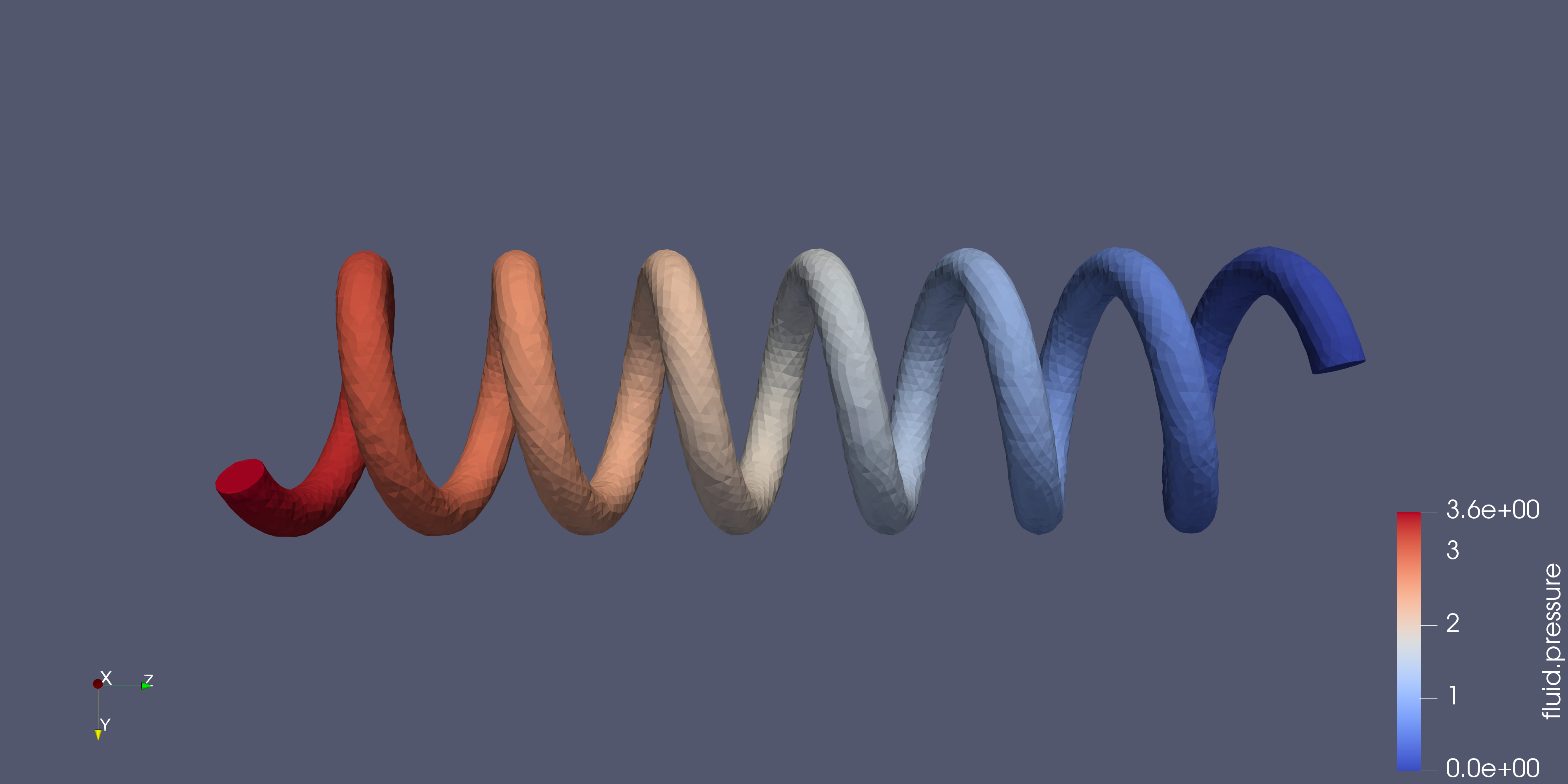
The geometry consists of a 7-turn coil spring shaped tube with one inlet and one outlet. The spring is 4.5cm long and its radius is 1cm. The tube’s radius is 1mm.
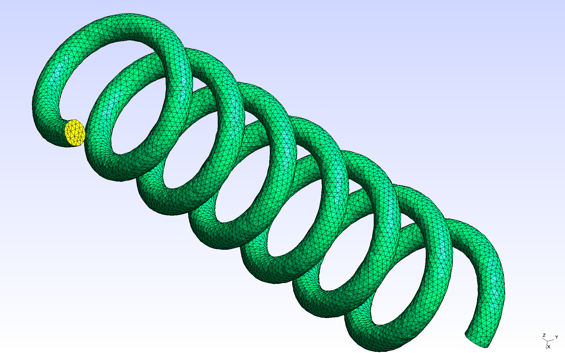
The mesh is available on Girder
5. Input parameters
| Name | Description | Value | Unit | |
|---|---|---|---|---|
\(\mu_f\) |
fluid viscosity |
\(6 \times 10^{-3}\) |
\(Pa.s\) |
|
\(\rho_f\) |
fluid density |
\(1056\) |
\(kg/m^3\) |
6. Reynolds number
Given the tube diameter \(D = 1 \times 10^{-3}m\), the fluid’s viscosity and density in the table above and the maximum inflow velocity (~0.7mm/s), we can calculate the Reynolds number:
\(R_e = \frac{\rho_f UD}{\mu_f} = \frac{1056 \times 7 \times 10^{-7}}{(6 \times 10^{-3})} \approx 1 \times 10^{-1} < 1\).
The Reynolds number is significantly lower than 1, which means we can use the Stokes model.
7. Model & Toolbox
The Stokes model for laminar flows is described in the CFD toolbox, see Computational Fluid Dynamics
7.1. Materials
  "Materials":
  {
    "lumenVolume":{
      "name":"Blood",
      "rho":1056, // [kg/m^3]
      "mu":6e-3 // [Pa.s]
    }
  },
7.2. Boundary conditions
The domain boundary are splitted in three parts: the inlet, the outlet and the wall of the tube. The wall is the part of the fluid domain boundary which corresponds to the tube, which is a solid.
7.2.1. Wall
We apply a Dirichlet boundary condition on the spring wall (fluid velocity vanishes near the wall). This means the fluid particles in contact with the wall are considered stuck on the (solid) tube, which implies the velocity of the fluid at the fluid-solid interface is the velocity of the solid boundary. Since we are only simulating the fluid flow, the tube is considered a non moving rigid body: it can not be deformed. Hence, its velocity at all point is zero, and so is the fluid velocity on the wall.
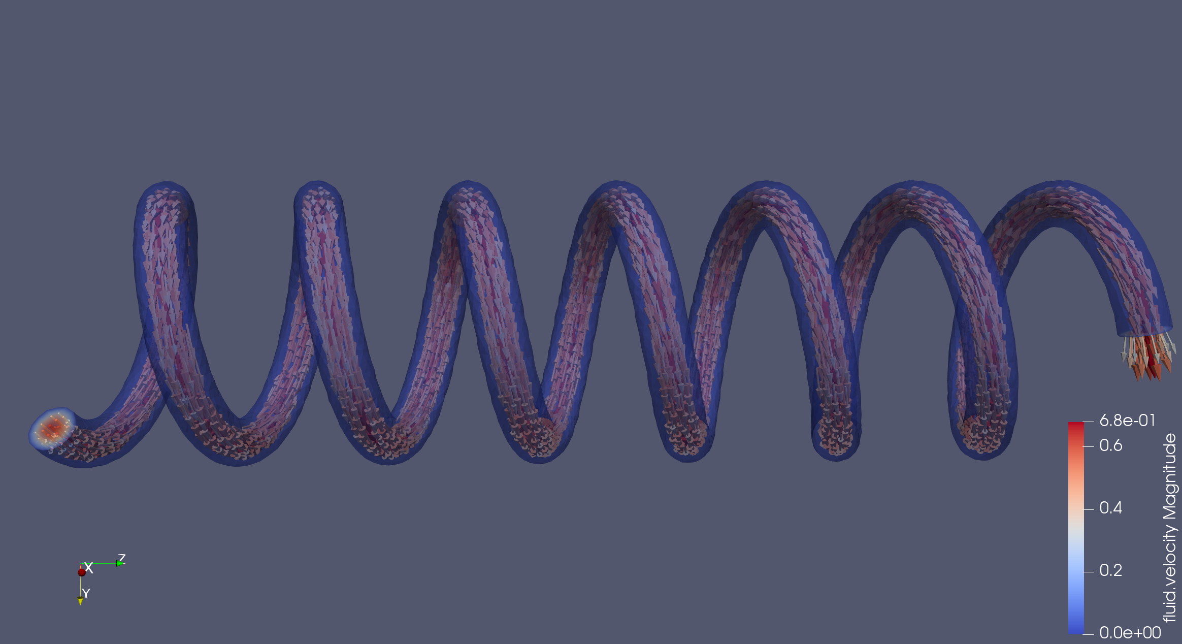
7.2.2. Inlet
For the inlet, we also use a Dirichlet condition: a parabolic shaped velocity profile is imposed with a given flow rate. The parabolic inflow corresponds to a Poiseuille law, which is valid for relatively thin and long tubes, with relatively low velocities (laminar flows). The Poiseuille law does not hold near the entrance of a real tube. Here, we assume the tube actually starts "before" our inlet, which could be seen as a virtual cut somewhere in a longer tube.
7.2.3. Outlet
The outlet is left with a free outflow boundary condition, which means no imposed stress along the normal to the boundary.
"BoundaryConditions":
{
"velocity":
{
"Dirichlet":
{
"wall":
{
"expr":"{0,0,0}"
}
}
},
"fluid":
{
"inlet":
{
"markerBottom":
{
"expr":"1e-9", // m^3/s
"shape":"parabolic", // constant, parabolic,
"constraint":"flow_rate" // velocity_max, flow_rate
}
}
}
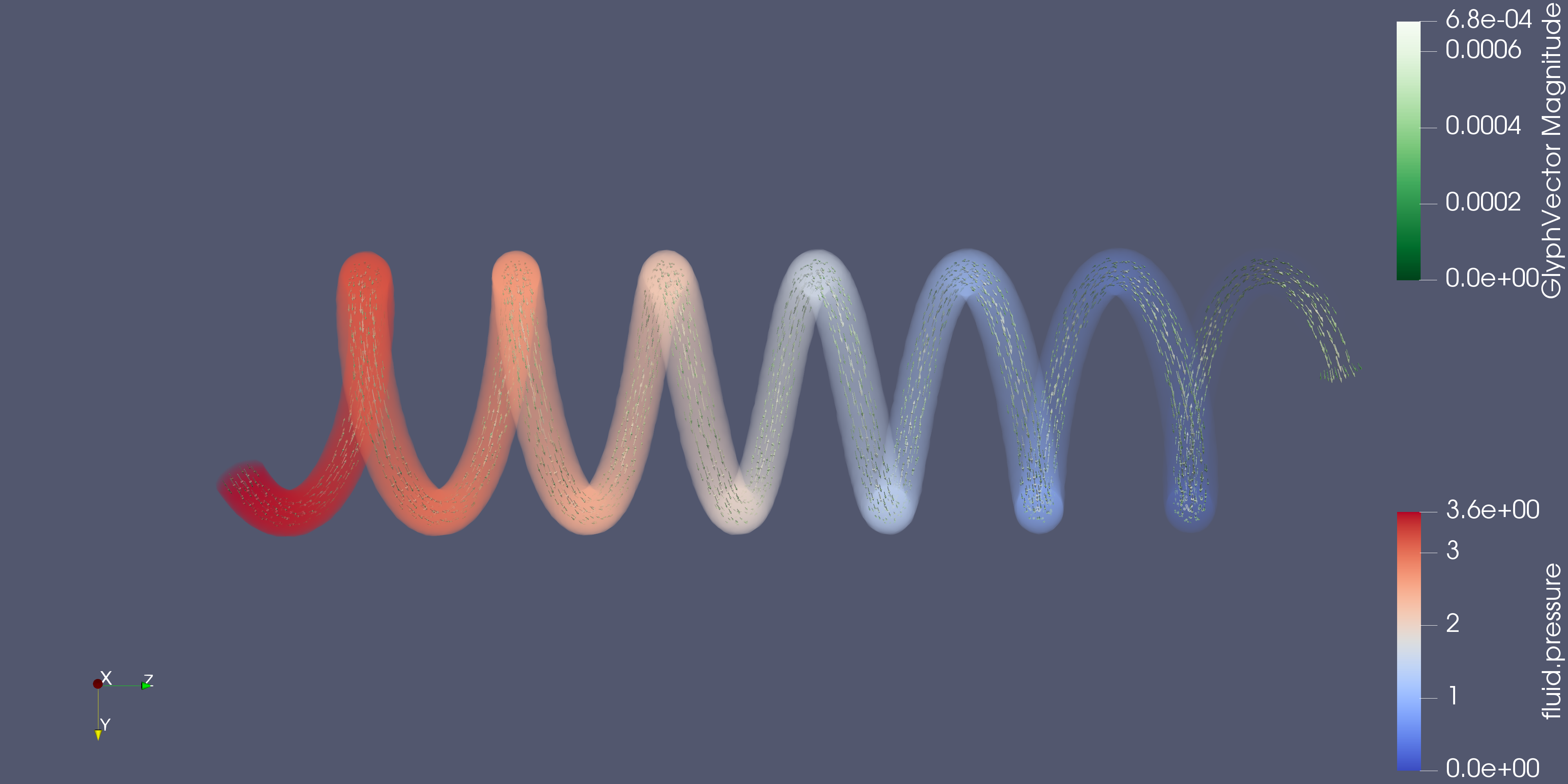
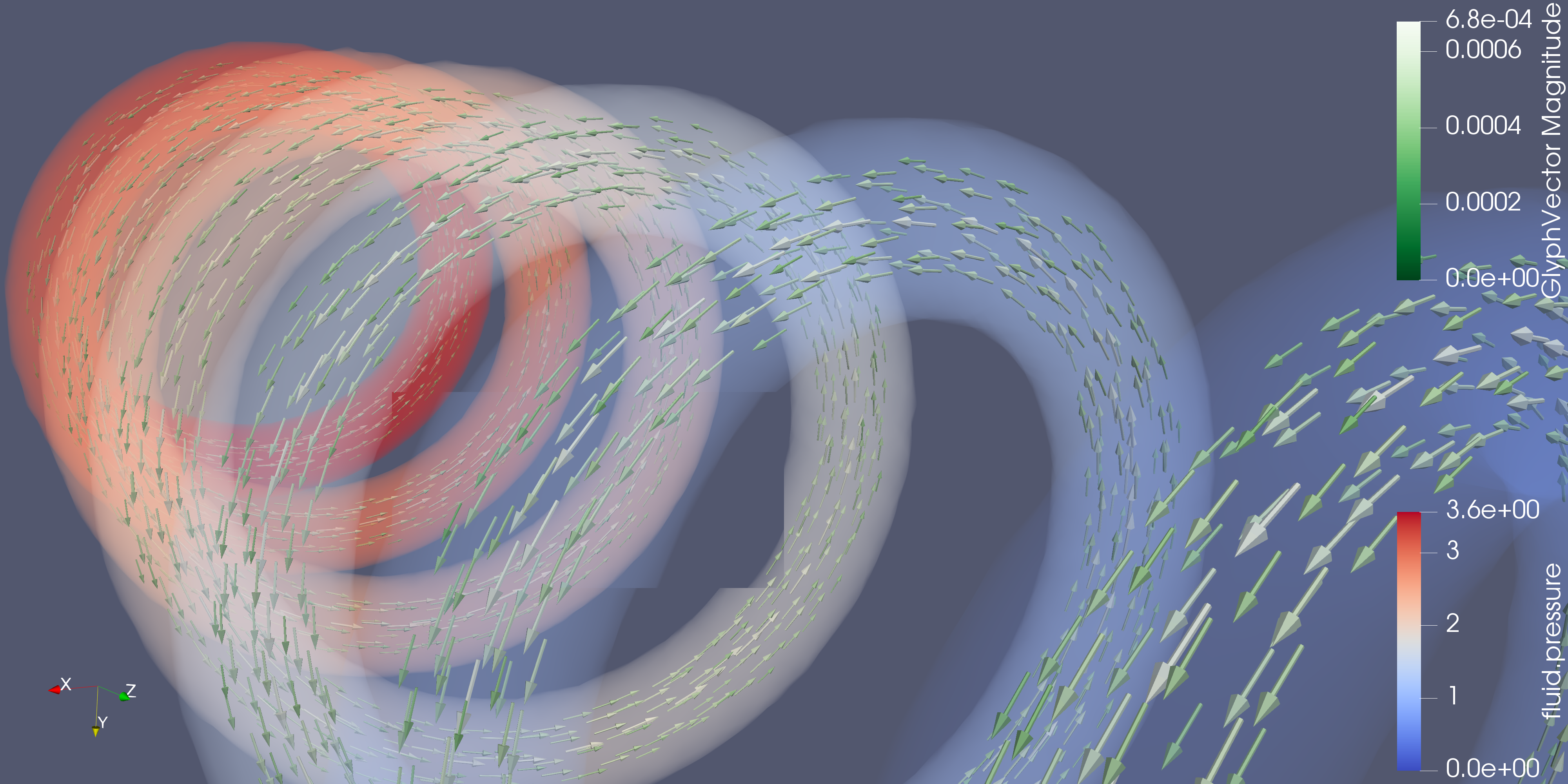
},8. Results
The fields of interest for this example are the velocity, the pressure of the fluid and the parallel process id (pid). The pid helps to see how the mesh was partitioned for parallel processing. In the 3D view below, when selecting the pid in the first dropdown list, each color corresponds to a subdomain assigned to and processed by a CPU core.