.pdf
.pdf
Examples of 2D Darcy flows
The following two examples come from [BD].
1. Example : 2D Darcy flow, chessboard pressure
1.1. Input parameters
| Notation | Quantity | Type | Unit |
|---|---|---|---|
\(\underline{\underline\kappa}\) |
Permeability |
order 2 tensor |
\(m^2Pa^{-1}s^{-1}\) |
\(f(x,y)\) |
Flux source term |
scalar function |
\(s^{-1}\) |
1.2. Model & Toolbox
We consider a 2D unit square \(\Omega=[0,1]\times[0,1]\) whose boundary is denoted \(\Gamma\). The following problem is to be solved in \(\Omega\).
with the additional condition \(\int_\Omega f=0\). The pressure is denoted \(p\) and the velocity \(\underline u\). We assume the material permeability is constant, isotropic and unitary, that is \(\underline{\underline\kappa}=\underline{\underline{I_d}}\).
Let us define the source term \(f=\nabla\cdot\underline u=-\Delta p\) to get the analytic solution \(p(x,y)=sin(2\pi x)cos(2\pi y)\). It yields \(f(x,y)=8\pi^2sin(2\pi x)cos(2\pi y)\).
This example runs within the Mixed Poisson toolbox with prescribed parameters.
1.3. Boundary conditions
We impose a Dirichlet boundary condition on the whole boundary : \(p=sin(2\pi x)cos(2\pi y)\text{ on }\Gamma\).
1.5. Convergence analysis
| \(h\) | 0.2 | 0.1 | 0.05 | 0.01 | 0.005 |
|---|---|---|---|---|---|
\(\Vert p-p_h\Vert_{L^2}\) |
9.57939e-01 |
5.42923e-01 |
2.78594e-01 |
5.6416e-02 |
2.83271e-02 |
\(\Vert u-u_h\Vert_{L^2}\) |
2.78314e-01 |
1.35505e-01 |
6.61506e-02 |
1.30739e-02 |
6.52889e-03 |
| \(h\) | 0.2 | 0.1 | 0.05 | 0.01 | 0.005 |
|---|---|---|---|---|---|
\(\Vert p-p_h\Vert_{L^2}\) |
1.69091e-01 |
4.85275e-02 |
1.26349e-02 |
5.14523e-04 |
1.28986e-04 |
\(\Vert u-u_h\Vert_{L^2}\) |
1.66947e-01 |
4.78222e-02 |
1.22767e-02 |
4.92702e-04 |
1.23431e-04 |
| \(h\) | 0.2 | 0.1 | 0.05 | 0.01 | 0.005 |
|---|---|---|---|---|---|
\(\Vert p-p_h\Vert_{L^2}\) |
2.22396e-02 |
3.15292e-03 |
4.07591e-04 |
3.22962e-06 |
4.0602e-07 |
\(\Vert u-u_h\Vert_{L^2}\) |
1.73431e-02 |
2.35603e-03 |
3.01594e-04 |
2.33871e-06 |
2.93291e-07 |
| \(h\) | 0.2 | 0.1 | 0.05 | 0.01 | 0.005 |
|---|---|---|---|---|---|
\(\Vert p-p_h\Vert_{L^2}\) |
2.03629e-03 |
1.52963e-04 |
9.81156e-06 |
1.56186e-08 |
9.80369e-10 |
\(\Vert u-u_h\Vert_{L^2}\) |
1.37478e-03 |
1.01811e-04 |
6.43878e-06 |
1.00732e-08 |
6.3051e-10 |
1.6. Output
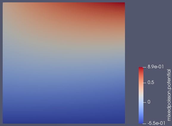
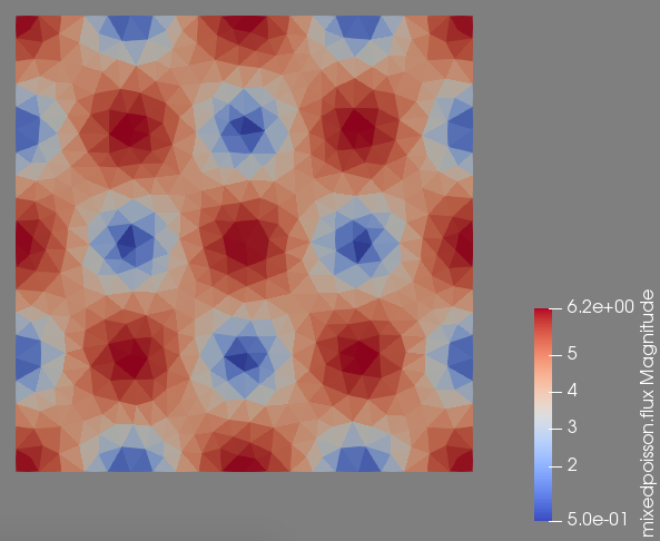
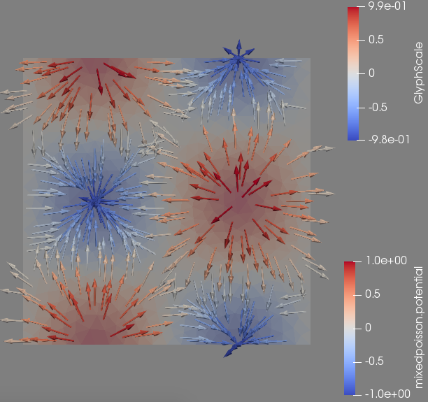
The following output example is reproducible using feelpp_toolbox_mixed-poisson-model_2DP2 running on 12 cores with the previous .json and .cfg files on a mesh of typical size \(h=0.05\).
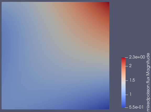
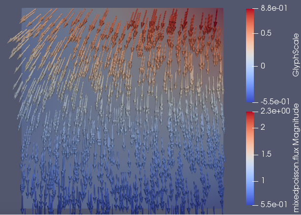
The screenshots are in order : the pressure field, the velocity magnitude field and the velocity field.
|
|
|
1.7. Example : Darcy flow, shower
The input parameters, model and toolbox are the same as in the previous example.
1.8. Boundary conditions
We impose a Dirichlet boundary condition on the whole boundary : \(p=sin(y)sin(x)+xy^2-\frac16-\sin(1)(1-\cos(1))\text{ on }\Gamma\).
1.10. Convergence analysis
| \(h\) | 0.2 | 0.1 | 0.05 | 0.01 | 0.005 |
|---|---|---|---|---|---|
\(\Vert p-p_h\Vert_{L^2}\) |
5.34577e-02 |
2.79542e-02 |
1.42528e-02 |
2.85709e-03 |
1.43102e-03 |
\(\Vert u-u_h\Vert_{L^2}\) |
4.78442e-02 |
2.43738e-02 |
1.23471e-02 |
2.45374e-03 |
1.22648e-03 |
| \(h\) | 0.2 | 0.1 | 0.05 | 0.01 | 0.005 |
|---|---|---|---|---|---|
\(\Vert p-p_h\Vert_{L^2}\) |
1.97729e-03 |
5.33807e-04 |
1.34873e-04 |
5.41901e-06 |
1.35843e-06 |
\(\Vert u-u_h\Vert_{L^2}\) |
6.14894e-03 |
1.61917e-03 |
3.99372e-04 |
1.52692e-05 |
3.81444e-06 |
| \(h\) | 0.2 | 0.1 | 0.05 | 0.01 | 0.005 |
|---|---|---|---|---|---|
\(\Vert p-p_h\Vert_{L^2}\) |
1.40696e-05 |
1.91059e-06 |
2.46414e-07 |
1.95803e-09 |
2.45484e-10 |
\(\Vert u-u_h\Vert_{L^2}\) |
5.16536e-05 |
7.12397e-06 |
9.13825e-07 |
7.16198e-09 |
8.98457e-10 |
| \(h\) | 0.2 | 0.1 | 0.05 | 0.01 | 0.005 |
|---|---|---|---|---|---|
\(\Vert p-p_h\Vert_{L^2}\) |
2.47985e-07 |
1.81459e-08 |
1.16742e-09 |
1.80373e-12 |
2.89473e-13 |
\(\Vert u-u_h\Vert_{L^2}\) |
6.13595e-07 |
4.34515e-08 |
2.77315e-09 |
4.19972e-12 |
1.17702e-12 |
1.11. Output
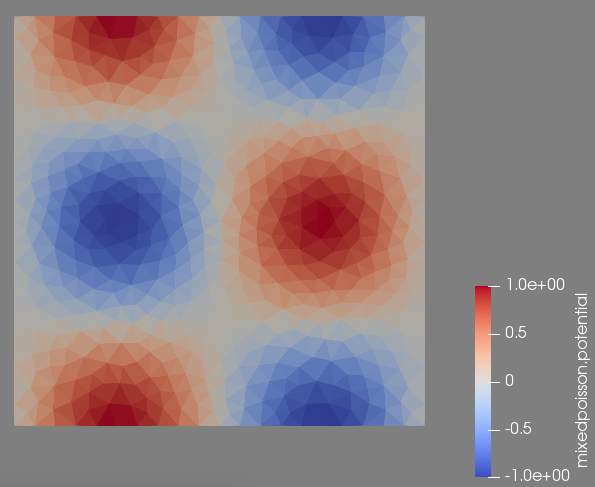
The following output example is reproducible using feelpp_toolbox_mixed-poisson-model_2DP2 running on 12 cores with the previous .json and .cfg files on a mesh of typical size \(h=0.05\).
The screenshots are in order : the pressure field, the velocity magnitude field and the velocity field.
|
|
|