Wave Pressure 2D

This test case has originally been realised by [Pena], [Nobile] and [GerbeauVidrascu] only with the free outlet condition.

Computer codes, used for the acquisition of results, are from Vincent [Chabannes]

1. Problem Description

We interest here to the case of bidimensional blood flow modelisation. We want to reproduce and observe pressure wave spread into a canal with a fluid-structure interaction model.

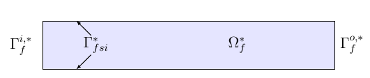
Figure 1 : Geometry of two-dimension elastic tube.

The figure above shows us the initial geometry we will work on. The canal is represent by a rectangle with width and height, respectively equal to 6 and 1 cm. The upper and lower walls are mobile and so, can be moved by flow action.

By using the 1D reduced model, named generalized string and explained by [Chabannes], we didn’t need to define the elastic domain ( for the vascular wall ) here. So the structure domain is \(\Omega_s^*=\Gamma_{fsi}^*\)

During this benchmark, we will compare two different cases : the free outlet condition and the Windkessel model. The first one, as its name said, impose a free condition on the fluid at the end of the domain. The second one is used to model more realistically an flow outlet into our case. The chosen time step is \(\Delta t=0.0001\)

1.1. Boundary conditions

We set :

on \(\Gamma_f^{i,*}\) the pressure wave pulse \[ \boldsymbol{\sigma}_{f} \boldsymbol{n}_f = \left\{ \begin{aligned} & \left(-\frac{2 \cdot 10^4}{2} \left( 1 - \cos \left( \frac{ \pi t} {2.5 \cdot 10^{-3}} \right) \right), 0\right)^T \quad & \text{ if } t < 0.005 \\ & \boldsymbol{0} \quad & \text{ else } \end{aligned} \right. \]
on \(\Gamma_f^{o,*}\)
- Case 1 : free outlet : \(\boldsymbol{\sigma}_{f} \boldsymbol{n}_f =0\)
- Case 2 : Windkessel model ( \(P_0\) proximal pressure, see [Chabannes] ) : \(\boldsymbol{\sigma}_{f} \boldsymbol{n}_f = -P_0\boldsymbol{n}_f\)
on \(\Gamma_f^{i,*} \cup \Gamma_f^{o,*}\) a null displacement : \(\boldsymbol{\eta}_f=0\)
on \(\Gamma^*_{fsi}\) : \(\eta_s=0\)
We add also the specific coupling conditions, obtained from the axisymmetric reduced model, on \(\Gamma^*_{fsi}\)

\[\dot{\eta}_s \boldsymbol{e}_r - \boldsymbol{u}_f = \boldsymbol{0}\]

\[f_s + \left(J_{\mathcal{A}_f^t} \boldsymbol{F}_{\mathcal{A}_f^t}^{-T} \hat{\boldsymbol{\sigma}}_f \boldsymbol{n}^*_f\right) \cdot \boldsymbol{e}_r = 0\]

\[\boldsymbol{\varphi}_s^t - \mathcal{A}_f^t = \boldsymbol{0}\]

1.2. Initial conditions

2. Inputs

Table 1. Fixed and Variable Input Parameters
Name	Description	Nominal Value	Units
\(E_s\)	Young’s modulus	\(0.75\)	\(dynes.cm^{-2}\)
\(\nu_s\)	Poisson’s ratio	\(0.5\)	dimensionless
\(h\)	walls thickness	0.1	\(cm\)
\(\rho_s\)	structure density	\(1.1\)	\(g.cm^{-3}\)
\(R_0\)	tube radius	\(0.5\)	\(cm\)
\(G_s\)	shear modulus	\(10^5\)	\(Pa\)
\(k\)	Timoshenko’s correction factor	\(2.5\)	dimensionless
\(\gamma_v\)	viscoelasticity parameter	\(0.01\)	dimensionless
\(\mu_f\)	viscosity	\(0.003\)	\(poise\)
\(\rho_f\)	density	\(1\)	\(g.cm^{-3}\)
\(R_p\)	proximal resistance	\(400\)
\(R_d\)	distal resistance	\(6.2 \times 10^3\)
\(C_d\)	capacitance	\(2.72 \times 10^{-4}\)

3. Outputs

After solving the fluid struture model, we obtain \((\mathcal{A}^t, \boldsymbol{u}_f, p_f, \boldsymbol{\eta}_s)\)

with \(\mathcal{A}^t\) the ALE map, \(\boldsymbol{u}_f\) the fluid velocity, \(p_f\) the fluid pressure and \(\boldsymbol\eta_s\) the structure displacement

4. Discretization

\(\mathcal{F}\) is the set of all mesh faces, we denote \(\mathcal{F}_{stab}\) the face we stabilize

\[\mathcal{F}_{stab} = \mathcal{F} \bigcap \left( \left\{ (x,y) \in \mathrm{R}^2: (x - 0.3) \leqslant 0 \right\} \cup \left\{ (x,y) \in \mathrm{^2: (x - 5.7) } \geqslant 0 \right\} \right)\]

In fact, after a first attempt, numerical instabilities can be observed at the fluid inlet. These instabilities, caused by pressure wave, and especially by the Neumann condition, make our fluid-structure solver diverge.

To correct them, we choose to add a stabilization term, obtain from the stabilized CIP formulation ( see [Chabannes], Chapter 6 ).

As this stabilization bring an important cost with it, by increasing the number of non-null term into the problem matrix, we only apply it at the fluid entrance, where the instabilities are located.

Now we present the different situations we worked on.

Config

Fluid

Structure

\(N_{elt}\)

\(N_{geo}\)

\(N_{dof}\)

\(N_{elt}\)

\(N_{geo}\)

\(N_{dof}\)

\((1)\)

\(342\)

\(3~(P4P3)\)

\(7377\)

\(58\)

\(1\)

\(176~(P3)\)

\((2)\)

\(342\)

\(4~(P5P4)\)

\(11751\)

\(58\)

\(1\)

\(234~(P4)\)

For the fluid time discretization, BDF, at order \(2\), is the method we use.

And Newmark-beta method is the one we choose for the structure time discretization, with parameters \(\gamma=0.5\) and \(\beta=0.25\).

These methods can be retrieved in [Chabannes] papers.

4.1. Solvers

Here are the different solvers ( linear and non-linear ) used during results acquisition.

KSP

case

fluid

solid

type

gmres

relative tolerance

\(1e-13\)

max iteration

\(30\)

\(10\)

reuse preconditioner

true

false

SNES

case

fluid

solid

relative tolerance

\(1e-8\)

steps tolerance

\(1e-8\)

max iteration

\(50\)

max iteration with reuse

\(50\)

reuse jacobian

false

reuse jacobian rebuild at first Newton step

false

true

KSP in SNES

case

fluid

solid

relative tolerance

\(1e-5\)

max iteration

\(1000\)

max iteration with reuse

\(1000\)

reuse preconditioner

true

false

reuse preconditioner rebuild at first Newton step

false

case

fluid

solid

type

package

mumps

FSI

solver method

fix point

tolerance

\(1e-6\)

max iterations

\(1\)

5. Results

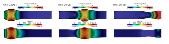
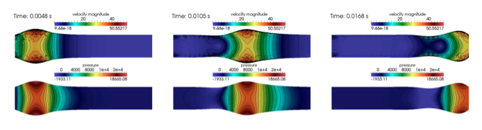
The two following pictures have their pressure and velocity magnitude amplify by 5.

Figure 2 : Results with free outlet conditon

Figure 3 : Results with the Windkessel model

Figure 4 : Evolution of the inflow and the outflow

Figure 5 : Maximum displacement magnitude

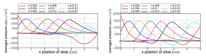
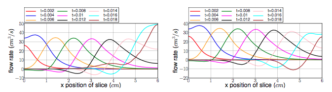
To draw the next two figures, we define 60 sections \(\{x_i\}_{i=0}^{60}\) with \(x_i=0.1i\).

Figure 5 : Average pressure with the free outlet and the Windkessel model

Figure 7 : Flow rate with the free outlet and the Windkessel model

Figure 8 : Implicit and semi-implicit FSI coupling comparison

Figure 9 : Implicit and semi-implicit FSI coupling comparison

All the files used for this case can be found in this rep [geo file, config file, fluid json file, solid json file].

5.1. Conclusion

Let’s begin with results with the free outlet condition ( see figure 2 ). These pictures show us how the pressure wave progresses into the tube. We can denote an increase of the fluid velocity at the end of the tube. Also, the wave eases at the same place. For the simulation with the Windkessel model, we observe a similar comportment at the beginning ( see figure 3 ). However, the outlet is more realistic than before. In fact, the pressure seems to propagate more naturally with this model. + In the two cases, the velocity field is disturbed at the fluid-structure interface. A mesh refinement around this region increases the quality. However, this is not crucial for the blood flow simulation.

Now we can interest us to the quantitative results.

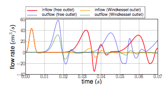
The inflow and outflow evolution figure ( see figure 4 ) shows us similarities for the two tests at the inlet. At the outlet, in contrast, the flow increases for the free outlet condition. In fact, when the pressure wave arrived at the outlet of the tube, it is reflected to the other way. In the same way, when the reflected wave arrived at the inlet, it is reflected again. The Windkessel model reduce significantly this phenomenon. Some residues stay due to 0D coupling model and structure fixation.

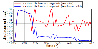
We also have calculate the maximum displacement magnitude for the two model ( see figure 5 ). The same phenomenons explained ahead are retrieve here. We denote that, for the free outlet, the structure undergoes movements during the test time, caused by the wave reflection. The Windkessel model reduces these perturbations thanks to the 0D model.

The average pressure and the fluid flow ( see figure 6 and 7 ) show us the same non-physiological phenomenons as before. The results we obtain are in accordance with the ones proposed by [Nobile].

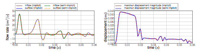
To end this benchmark, we will compare the two resolution algorithms used with the fluid-structure model : the implicit and the semi-implicit ones. The second configuration with Windkessel model is used for the measures.

We have then the fluid flow and the displacement magnitude ( figure 8 ) curves, which superimposed on each other. So the accuracy obtained by the semi-implicit method seems good here.

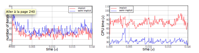
The performances of the two algorithms ( figure 9 ) are expressed from number of iterations and CPU time at each step time. The semi-implicit method is a bit ahead of the implicit one on number of iterations. However, the CPU time is smaller for 2 or 3 time, due to optimization in this method. First an unique ALE map estimation is need. Furthermore, linear terms of the Jacobian matrix, residuals terms and dependent part of the ALE map can be stored and reused at each iteration.

6. Bibliography

References for this benchmark

[Pena] G. Pena, Spectral element approximation of the incompressible Navier-Stokes equations evolving in a moving domain and applications, École Polytechnique Fédérale de Lausanne, November 2009.
[Nobile] F. Nobile, Numerical approximation of fluid-structure interaction problems with application to haemodynamics, École Polytechnique Fédérale de Lausanne, Switzerland, 2001.
[GerbeauVidrascu] J.F. Gerbeau, M. Vidrascu, A quasi-newton algorithm based on a reduced model for fluid-structure interaction problems in blood flows, 2003.
[Chabannes] Vincent Chabannes, Vers la simulation numérique des écoulements sanguins, Équations aux dérivées partielles [math.AP], Université de Grenoble, 2013.