 .pdf
.pdf
Cantilever CSM Benchmark
1. Introduction
We realize here a benchmark on the deformation of an elastic structure, initially the Cantilever problem, we simulate a simple cantilevered beam with a fixed end and a load applied to the other end. We will compare the obtained results with different meshes and a different polynomial degree in order to evaluate the time resolution.
2. Running the model
The configuration file are in benchmarks/modules/csm/examples/cantilever.
Some useful commande lines:
To executing Cantilever testcase
mpirun -np 4 feelpp_toolbox_solid --case "github:{repo:toolbox,path:examples/modules/csm/pages/cantilever}"Some useful command lines:
To edit the mesh step for 0.5 we must add
--gmsh.hsize= 0.5
To edit polynomial degree we must add
--case.discretization=P1
3. Model
We consider a Linear-Elasticity model.
4. Geometry
We consider a solid structure, composed of an elastic bar, which is fixed on one side that we note \(\Gamma_{L}\) (F:fixed) resulting in the displacement \(\boldsymbol{\eta}_s=0\) on the edges of \(\Omega_s\) and a load applied to the other end that we note \(\Gamma_{L}=\partial\Omega_s \backslash \Gamma_F\).
The geometry can be represented as follows:
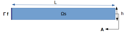
In this case test, we will observe the behavior of \(A\), during this simulation, we will obtain the displacement of \(A\), on the axis \(x\) and \(y\) , when the elastic structure is subjected to its own weight and a hanging weight to her.
5. Input parameters
5.1. Boundary conditions
We set
-
On \(\Gamma_{F}\),a condition that imposes this boundary to be fixed : \(\boldsymbol{\eta}_s=0\) (ps: \(\boldsymbol{\eta}_s\) is the displacement )
-
On \(\Gamma_{L}\), a force will be applied on the other end of the beam.
5.2. Discretization
To solve this problem we will use the Feel++ Toolboxes that use Finite Elements Method, with Lagrangian elements of order \(N\) to discretize space.
There are several different Toolboxes available, such as: CSM, CFD, Heat Transfer, etc. Of these, we need the CSM (Computational Solid Mechanics) Toolbox.
It is also necessary to define the type of the simulation. For example “Elasticity” is generally applied in case of metals, and “Hyper-Elasticity” for plastics.
5.3. Solvers
Here are the different solvers (linear) used during results acquisition.
type |
cg |
relative tolerance |
1e-8 |
max iteration |
1000 |
reuse preconditioner |
true |
type |
gamg |
package |
PETSC |
-
Regarding the resolution, we used the conjugate gradient method with the mutligrille preconditioner, because we are working on a linear system.
5.4. Parameters
The following table displays the material properties of the model.We will use the following data:
Name |
Description |
Nominal Value |
Units |
\(g\) |
gravitational constant |
2 |
\(m / s^2\) |
\(l\) |
elastic structure length |
\(40\) |
\(m\) |
\(h\) |
elastic structure height |
\(8\) |
\(m\) |
\(E_s\) |
Young’s modulus |
\(206.84277e9\) |
\(kg / ms^2\) |
\(\nu_s\) |
Poisson’s ratio |
\(0.3\) |
dimensionless |
\(\rho_s\) |
density |
\(7870\) |
\(kg/ m^3\) |
6. Outputs
As described before, in this problem, we try to determine the displacement \(\boldsymbol{\eta}_s\) on \(\Omega_s\), which verifies the following equation:
Add to this, the execution time as well as the degree of freedom and the number of element generated by the different steps of meshes and we will compare at the end the results with different meshes and a different polynomial degree in order to evaluate the time resolution.
7. References
-
Yousef Saad, Iterative Methods for Sparse Linear Systems, Second edition with correction. January 3rd, 2000.
-
[] Theory of solid mechanics : docs.feelpp.org/toolboxes/0.104/csm/theory/
-
[] Feel++ Toolboxes Manual : docs.feelpp.org/toolboxes/0.104/