 .pdf
.pdf
CFD Benchmarks
1. Introduction
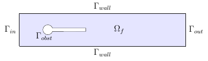
We implement the benchmark proposed by [TurekHron], on the behavior of drag and lift forces of a flow around an object composed by a pole and a bar, see Figure Geometry of the Turek & Hron CFD Benchmark.
The software and the numerical results were initially obtained from [Chabannes].
| This benchmark is linked to the Turek-Hron CSM and Turek-Hron FSI benchmarks. |
2. Problem Description
We consider a 2D model representative of a laminar incompressible flow around an obstacle. The flow domain, named \(\Omega_f\), is contained into the rectangle \( \lbrack 0,2.5 \rbrack \times \lbrack 0,0.41 \rbrack \). It is characterised, in particular, by its dynamic viscosity \(\mu_f\) and by its density \(\rho_f\). In this case, the fluid material we used is glycerine.
In order to describe the flow, the incompressible Navier-Stokes model is chosen for this case, define by the conservation of momentum equation and the conservation of mass equation. At them, we add the material constitutive equation, that help us to define \(\boldsymbol{\sigma}_f\)
The goal of this benchmark is to study the behavior of lift forces \(F_L\) and drag forces \(F_D\), with three different fluid dynamics applied on the obstacle, i.e on \(\Gamma_{obst}\), we made rigid by setting specific structure parameters. To simulate these cases, different mean inflow velocities, and thus different Reynolds numbers, will be used.
2.1. Boundary conditions
We set
-
on \(\Gamma_{in}\), an inflow Dirichlet condition : \( \boldsymbol{u}_f=(v_{in},0) \)
-
on \(\Gamma_{wall}\) and \(\Gamma_{obst}\), a homogeneous Dirichlet condition : \( \boldsymbol{u}_f=\boldsymbol{0} \)
-
on \(\Gamma_{out}\), a Neumann condition : \( \boldsymbol{\sigma}_f\boldsymbol{ n }_f=\boldsymbol{0} \)
2.2. Initial conditions
We use a parabolic velocity profile, in order to describe the flow inlet by \( \Gamma_{in} \), which can be express by
where \(\bar{U}\) is the mean inflow velocity.
However, we want to impose a progressive increase of this velocity profile. That’s why we define
With t the time.
Moreover, in this case, there is no source term, so \(f_f\equiv 0\).
3. Inputs
The following table displays the various fixed and variables parameters of this test-case.
| Name | Description | Nominal Value | Units | ||||||
|---|---|---|---|---|---|---|---|---|---|
\(l\) |
elastic structure length |
\(0.35\) |
\(m\) |
||||||
\(h\) |
elastic structure height |
\(0.02\) |
\(m\) |
||||||
\(r\) |
cylinder radius |
\(0.05\) |
\(m\) |
||||||
\(C\) |
cylinder center coordinates |
\((0.2,0.2)\) |
\(m\) |
||||||
\(\nu_f\) |
kinematic viscosity |
\(1\times 10^{-3}\) |
\(m^2/s\) |
||||||
\(\mu_f\) |
dynamic viscosity |
\(1\) |
\(kg/(m \times s)\) |
||||||
\(\rho_f\) |
density |
\(1000\) |
\(kg/m^3\) |
||||||
\(f_f\) |
source term |
0 |
\(kg/(m^3 \times s)\) |
||||||
\(\bar{U}\) |
characteristic inflow velocity |
|
\(m/s\) |
4. Outputs
As defined above, the goal of this benchmark is to measure the drag and lift forces, \(F_D\) and \(F_L\), to control the fluid solver behavior. They can be obtain from
where \(\boldsymbol{n}_f\) the outer unit normal vector from \(\partial \Omega_f\).
5. Discretization
To realize these tests, we made the choice to used \(P_N\)-\(P_{N-1}\) Taylor-Hood finite elements, described by [Chabannes], to discretize space. With the time discretization, we use BDF, for Backward Differentation Formulation, schemes at different orders \(q\).
6. Running the case
7. Data files
8. Results
Here are results from the different cases studied in this benchmark.
8.1. CFD1
| \(\mathbf{N_{geo}}\) | \(\mathbf{N_{elt}}\) | \(\mathbf{N_{dof}}\) | Drag | Lift |
|---|---|---|---|---|
Reference [TurekHron] |
14.29 |
1.119 |
||
1 |
9874 |
45533 (\(P_2/P_1\)) |
14.217 |
1.116 |
1 |
38094 |
173608 (\(P_2/P_1\)) |
14.253 |
1.120 |
1 |
59586 |
270867 (\(P_2/P_1\)) |
14.262 |
1.119 |
2 |
7026 |
78758 (\(P_3/P_2\)) |
14.263 |
1.121 |
2 |
59650 |
660518 (\(P_3/P_2\)) |
14.278 |
1.119 |
3 |
7026 |
146057 (\(P_4/P_3\)) |
14.270 |
1.120 |
3 |
59650 |
1228831 (\(P_4/P_3\)) |
14.280 |
1.119 |
All the files used for this case can be found in this rep [geo file, config file, json file]
8.2. CFD2
| \(\mathbf{N_{geo}}\) | \(\mathbf{N_{elt}}\) | \(\mathbf{N_{dof}}\) | Drag | Lift |
|---|---|---|---|---|
Reference [TurekHron] |
136.7 |
10.53 |
||
1 |
7020 |
32510 (\(P_2/P_1\)) |
135.33 |
10.364 |
1 |
38094 |
173608 (\(P_2/P_1\)) |
136.39 |
10.537 |
1 |
59586 |
270867 (\(P_2/P_1\)) |
136.49 |
10.531 |
2 |
7026 |
78758 (\(P_3/P_2\)) |
136.67 |
10.548 |
2 |
59650 |
660518 (\(P_3/P_2\)) |
136.66 |
10.532 |
3 |
7026 |
146057 (\(P_4/P_3\)) |
136.65 |
10.539 |
3 |
59650 |
1228831 (\(P_4/P_3\)) |
136.66 |
10.533 |
All the files used for this case can be found in this rep [geo file, config file, json file]
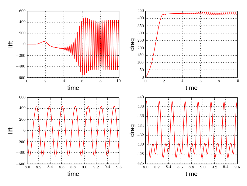
8.3. CFD3
As CFD3 is time-dependent ( from BDF use ), results will be expressed as
where
-
mean is the average of the min and max values at the last period of oscillations.
-
amplitude is the difference of the max and the min at the last oscillation.
-
frequency can be obtain by Fourier analysis on periodic data and retrieve the lowest frequency or by the following formula, if we know the period time T.
| \(\mathbf{\Delta t}\) | \(\mathbf{N_{geo}}\) | \(\mathbf{N_{elt}}\) | \(\mathbf{N_{dof}}\) | \(\mathbf{N_{bdf}}\) | Drag | Lift |
|---|---|---|---|---|---|---|
0.005 |
Reference [TurekHron] |
439.45 ± 5.6183[4.3956] |
−11.893 ± 437.81[4.3956] |
|||
0.01 |
1 |
8042 |
37514 (\(P_2/P_1\)) |
2 |
437.47 ± 5.3750[4.3457] |
-9.786 ± 437.54[4.3457] |
2 |
2334 |
26706 (\(P_3/P_2\)) |
2 |
439.27 ± 5.1620[4.3457] |
-8.887 ± 429.06[4.3457] |
|
2 |
7970 |
89790 (\(P_2/P_2\)) |
2 |
439.56 ± 5.2335[4.3457] |
-11.719 ± 425.81[4.3457] |
0.005 |
1 |
3509 |
39843\((P_3/P_2)\) |
2 |
438.24 ± 5.5375[4.3945] |
-11.024 ± 433.90[4.3945] |
1 |
8042 |
90582 (\(P_3/P_2\)) |
2 |
439.25 ± 5.6130[4.3945] |
-10.988 ± 437.70[4.3945] |
|
2 |
2334 |
26706 (\(P_3/P_2\)) |
2 |
439.49 ± 5.5985[4.3945] |
-10.534 ± 441.02[4.3945] |
|
2 |
7970 |
89790 (\(P_3/P_2\)) |
2 |
439.71 ± 5.6410[4.3945] |
-11.375 ± 438.37[4.3945] |
|
3 |
3499 |
73440 (\(P_4/P_3\)) |
3 |
439.93 ± 5.8072[4.3945] |
-14.511 ± 440.96[4.3945] |
|
4 |
2314 |
78168 (\(P_5/P_4\)) |
2 |
439.66 ± 5.6412[4.3945] |
-11.329 ± 438.93[4.3945] |
0.002 |
2 |
7942 |
89482 (\(P_3/P_2)\) |
2 |
439.81 ± 5.7370[4.3945] |
-13.730 ± 439.30[4.3945] |
3 |
2340 |
49389 (\(P_4/P_3\)) |
2 |
440.03 ± 5.7321[4.3945] |
-13.250 ± 439.64[4.3945] |
|
3 |
2334 |
49266 (\(P_4/P_3\)) |
3 |
440.06 ± 5.7773[4.3945] |
-14.092 ± 440.07[4.3945] |
All the files used for this case can be found in this rep [geo file, config file, json file].
10. Conclusion
The reference results of [TurekHron] have been obtained with a time step \(\Delta t=0.05\). When we compare our results, with the same step and \(\mathrm{BDF}_2\), we observe that they are in accordance with the reference results.
With a larger \(\Delta t\), a discrepancy is observed, in particular for the drag force. It can also be seen at the same time step, with a higher order \(\mathrm{BDF}_n\) ( e.g. \(\mathrm{BDF}_3\) ). This suggests that the couple \(\Delta t=0.05\) and \(\mathrm{BDF}_2\) isn’t enough accurate.
11. Bibliography
-
[TurekHron] S. Turek and J. Hron, Proposal for numerical benchmarking of fluid-structure interaction between an elastic object and laminar incompressible flow, Lecture Notes in Computational Science and Engineering, 2006.
-
[Chabannes] Vincent Chabannes, Vers la simulation numérique des écoulements sanguins, Équations aux dérivées partielles [math.AP], Universitée de Grenoble, 2013.