 .pdf
.pdf
2D Drops Benchmark
This benchmark has been proposed and realised by [Hysing]. It allows us to verify our level set code, our Navier-Stokes solver and how they couple together.
Computer codes, used for the acquisition of results, are from [Doyeux], with the use of [Chabannes]'s Navier-Stokes code.
1. Problem Description
We want to simulate the rising of a 2D bubble in a Newtonian fluid. The bubble, made of a specific fluid, is placed into a second one, with a higher density. Like this, the bubble, due to its lowest density and by the action of gravity, rises.
The equations used to define fluid bubble rising in an other are the Navier-Stokes for the fluid and the advection one for the level set method. As for the bubble rising, two forces are defined :
-
The gravity force : \(\boldsymbol{f}_g=\rho_\phi\boldsymbol{g}\)
-
The surface tension force : \(\boldsymbol{f}_{st}=\int_\Gamma\sigma\kappa\boldsymbol{ n } \)
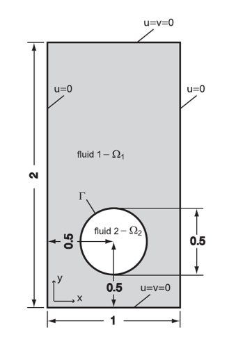
We denote \( \Omega\times\rbrack0,3\rbrack \) the interest domain with \( \Omega=(0,1)\times(0,2) \). \(\Omega\) can be decompose into \(\Omega_1\), the domain outside the bubble and \(\Omega_2\) the domain inside the bubble and \(\Gamma\) the interface between these two.
Durig this benchmark, we will study two different cases : the first one with a ellipsoidal bubble and the second one with a squirted bubble.
1.1. Boundary conditions
-
On the lateral walls, we imposed slip conditions
-
On the horizontal walls, no slip conditions are imposed : \(\boldsymbol{u}=0 \)
2. Inputs
The following table displays the various fixed and variables parameters of this test-case.
| Name | Description | Nominal Value | Units |
|---|---|---|---|
\(\boldsymbol{g}\) |
gravity acceleration |
\((0,0.98)\) |
\(m/s^2\) |
\(l\) |
length domain |
\(1\) |
\(m\) |
\(h\) |
height domain |
\(2\) |
\(m\) |
\(r\) |
bubble radius |
\(0.25\) |
\(m\) |
\(B_c\) |
bubble center |
\((0.5,0.5)\) |
\(m\) |
3. Outputs
In the first place, the quantities we want to measure are \(X_c\) the position of the center of the mass of the bubble, the velocity of the center of the mass \(U_c\) and the circularity \(c\), define as the ratio between the perimeter of a circle and the perimeter of the bubble. They can be expressed by
After that, we interest us to quantitative points for comparison as \(c_{min}\), the minimum of the circularity and \(t_{c_{min}}\), the time needed to obtain this minimum, \(u_{c_{max}}\) and \(t_{u_{c_{max}}}\) the maximum velocity and the time to attain it, or \(y_c(t=3)\) the position of the bubble at the final time step. We add a second maximum velocity \(u_{max}\) and \(u_{c_{max_2}}\) and its time \(t_{u_{c_{max_2}}}\) for the second test on the squirted bubble.
4. Discretization
This is the parameters associate to the two cases, which interest us here.
Case |
\(\rho_1\) |
\(\rho_2\) |
\(\mu_1\) |
\(\mu_2\) |
\(\sigma\) |
Re |
\(E_0\) |
ellipsoidal bubble (1) |
1000 |
100 |
10 |
1 |
24.5 |
35 |
10 |
squirted bubble (2) |
1000 |
1 |
10 |
0.1 |
1.96 |
35 |
125 |
6. Results
6.2. Test 2
We describe the different quantitative results for the two studied cases.
h |
\(c_{min}\) |
\(t_{c_{min}}\) |
\(u_{c_{max}}\) |
\(t_{u_{c_{max}}}\) |
\(y_c(t=3)\) |
lower bound |
0.9011 |
1.8750 |
0.2417 |
0.9213 |
1.0799 |
upper bound |
0.9013 |
1.9041 |
0.2421 |
0.9313 |
1.0817 |
0.02 |
0.8981 |
1.925 |
0.2400 |
0.9280 |
1.0787 |
0.01 |
0.8999 |
1.9 |
0.2410 |
0.9252 |
1.0812 |
0.00875 |
0.89998 |
1.9 |
0.2410 |
0.9259 |
1.0814 |
0.0075 |
0.9001 |
1.9 |
0.2412 |
0.9251 |
1.0812 |
0.00625 |
0.8981 |
1.9 |
0.2412 |
0.9248 |
1.0815 |
h |
\(c_{min}\) |
\(t_{c_{min}}\) |
\(u_{c_{max_1}}\) |
\(t_{u_{c_{max_1}}}\) |
\(u_{c_{max_2}}\) |
\(t_{u_{c_{max_2}}}\) |
\(y_c(t=3)\) |
lower bound |
0.4647 |
2.4004 |
0.2502 |
0.7281 |
0.2393 |
1.9844 |
1.1249 |
upper bound |
0.5869 |
3.0000 |
0.2524 |
0.7332 |
0.2440 |
2.0705 |
1.1380 |
0.02 |
0.4744 |
2.995 |
0.2464 |
0.7529 |
0.2207 |
1.8319 |
1.0810 |
0.01 |
0.4642 |
2.995 |
0.2493 |
0.7559 |
0.2315 |
1.8522 |
1.1012 |
0.00875 |
0.4629 |
2.995 |
0.2494 |
0.7565 |
0.2324 |
1.8622 |
1.1047 |
0.0075 |
0.4646 |
2.995 |
0.2495 |
0.7574 |
0.2333 |
1.8739 |
1.1111 |
0.00625 |
0.4616 |
2.995 |
0.2496 |
0.7574 |
0.2341 |
1.8828 |
1.1186 |
7. Bibliography
-
[Hysing] S. Hysing, S. Turek, D. Kuzmin, N. Parolini, E. Burman, S. Ganesan, and L. Tobiska, Quantitative benchmark computations of two-dimensional bubble dynamics, International Journal for Numerical Methods in Fluids, 2009.
-
[Chabannes] V. Chabannes, Vers la simulation numérique des écoulements sanguins, Équations aux dérivées partielles. PhD thesis, Université de Grenoble, 2013.
-
[Doyeux] V. Doyeux, Modélisation et simulation de systèmes multi-fluides, Application aux écoulements sanguins, PhD thesis, Université de Grenoble, 2014.