 .pdf
.pdf
Aerothermal Flow in an Airplane Cabin
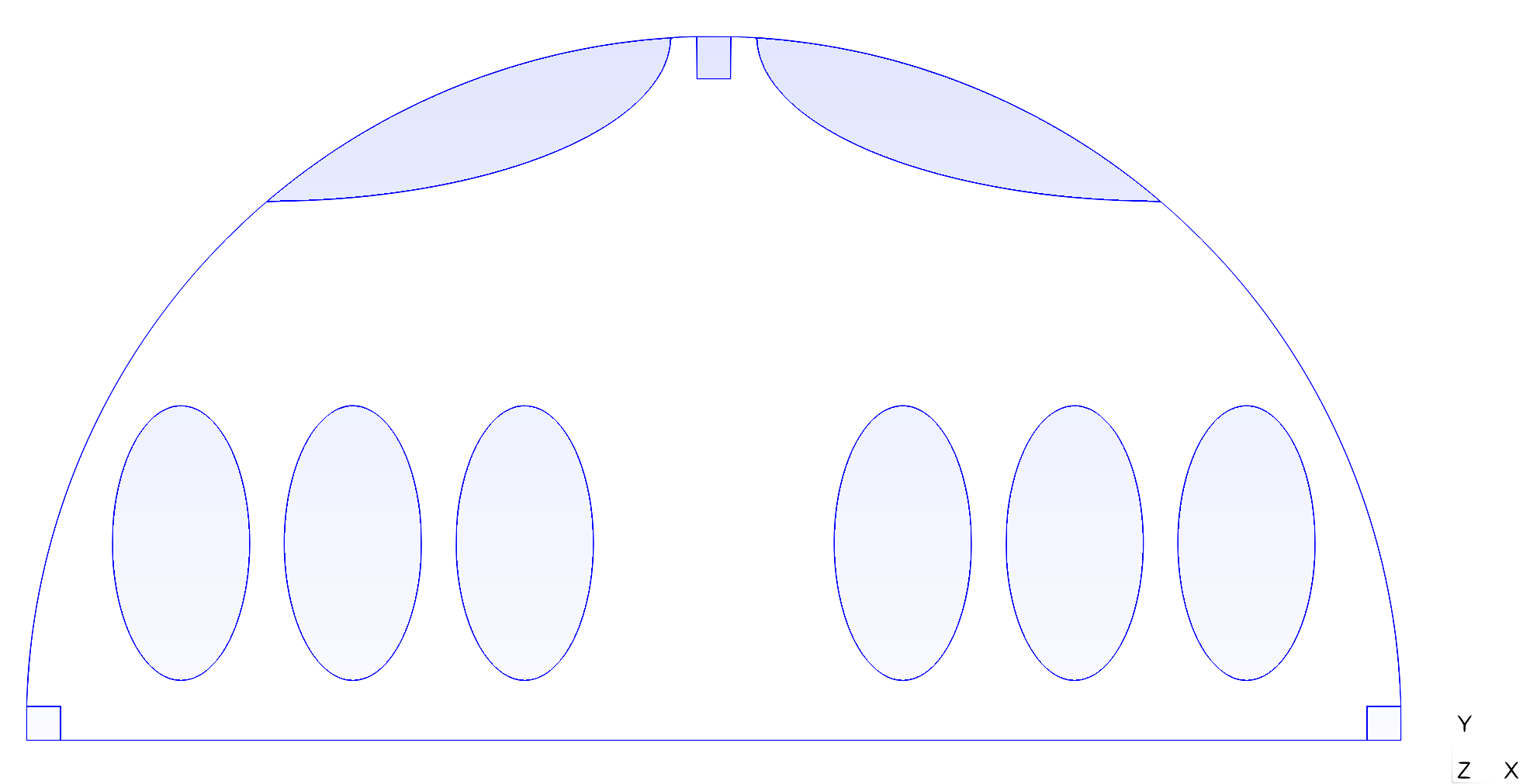
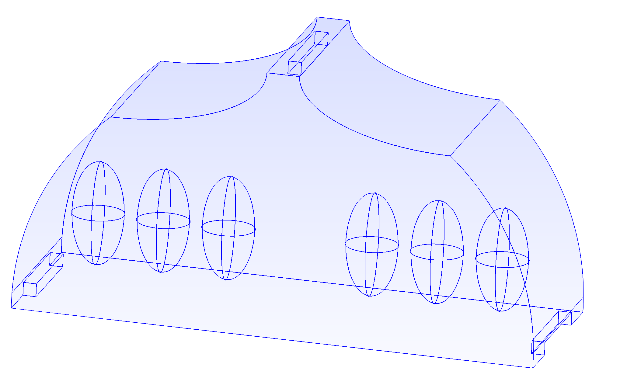
The aim of this example is to model the aerothermal flows in an airplane cabin. Cooling air is flowing in from the inlet on the top and flowing out in the two outlets at the bottom of the cabin. The six passengers are heating the domain with a constant heat flux.
This test case was proposed by Airbus Group. The interest of such simulation is to optimize the performances of the Environmental Constrol System (ECS). The ECS manage, among other things, the quality of the air. This equipment is crucial to guaranty the comfort and the security of the passengers. Performing accurate and efficient simulations on the present test case allows to optimize the ECS capabilities with two levers of actions. First, the numerical models can be used during the early phases of design and risk analysis, in order to optimize the cabin. Then, the 3D simulation can be used in an active way, coupled with the ECS, to predict the behaviour of the aerothermal fields in the airplane.
The physical hypothesis of the model are :
-
Incompressible fluid
-
Newtonian fluid
-
Boussinesq approximation to describe the buoyancy force
These assumptions lead to a coupled system between the Navier-Stokes equation for the fluid and an advection diffusion equation for the temperature. We refer the reader to the documentation of the HeatFluid toolbox for more details on this system of equations.
The following boundary conditions are applied:
-
For the fluid (velocity/pressure)
-
Dirichlet condition on the inlet with a Poiseuille profile of magnitude \(U_{in}\):
\[u=(0,-U_{in}600(0.05-x)(x+0.05))\] -
Free Stream condition on the outlets:
\[\mu\nabla u\cdot n-p n=0\] -
Homogeneous Dirichlet (no-slip) condition on all the others solid walls:
\[u=(0,0)\]
-
-
For the temperature:
-
A Dirichlet condition on the inlet:
\[T=T_{in}\] -
A Neumann condition (constant flux):
\[-k\nabla T\cdot n=C_p Q_{P},\] -
A homogeneous Neumann condition (insulated walls) on the other solid walls:
\[\nabla T\cdot n=0\]
-
This example can be run on a 2D or a 3D geometry. We detail the input data for both configuration in the following paragraphs.
1. Running the case
The commande line to run this case is: in 2D
mpirun -np 4 feelpp_toolbox_heatfluid --case "github:{repo:toolbox,path:examples/modules/heatfluid/examples/cabin}"in 3D
mpirun -np 4 feelpp_toolbox_heatfluid --case "github:{repo:toolbox,path:examples/modules/heatfluid/examples/cabin}" --case.config-file cabin3d.cfg3. Geometry
The geometry is an simplified cut of the cabin. The passengers are modeled by the six egg-shaped objects
2D Geometry
3D Geometry
4. Input Parameters
| Name | Description | Value | Unit | |
|---|---|---|---|---|
\(U_{in}\) |
Amplitude of the velocity at the inlet |
0.75 |
\(m.s^{-1}\) |
|
\(T_{in}\) |
Temperature of the fluid at the inlet |
288,15 |
\(K\) |
"Parameters":
{
    "Uin":0.75,
    "Tin":15
},
5. Materials
We consider a fluid in all the domain. We use a smooth approximation of the real physical parameters of the air in order to model the turbulent loss of energy in the small scales.
| Name | Description | Value | Unit | |
|---|---|---|---|---|
\(\rho\) |
Density |
\(1\) |
\(kg.m^{-3}\) |
|
\(\mu\) |
Dynamic viscosity |
\(5.0\cdot 10^{-4}\) |
\(kg.m^{−1}.s^{-1}\) |
|
\(k\) |
Thermal conductivity |
\(1.45\cdot 10^{-2}\) |
\(W.m^{-1}.K^{-1}\) |
|
\(C_p\) |
Heat capacity |
stem::[1000] |
\(J.kg^{-1}.K^{-1}\) |
|
\(\beta\) |
Coefficient of thermal expansion |
\(0.003660\) |
\(K^{-1}\) |
"Materials":
{
    "Fluid":{
        "rho":"1.0",
        "mu":"5.0e-4",
        "k":"1.45e-2",
        "Cp":"1000",
        "beta":"0.003660" //0.00006900
    }
},
6. Boundary Conditions
We impose a standard no-slip condition on all the solid walls and on the passengers (homogeneous Dirichlet). The flow at the inlet it modeled by a poiseuille profile (Dirichlet). At the outlet we impose a do nothing (Neumann) condition.
"velocity":
{
    "Dirichlet":
    {
        "inlet" : {"expr":"{0,-Uin*(0.05-x)*(x+0.05)*400*(1-exp(-5*t)),0}:x:y:z:t:Uin"},
        "passengers" : {"expr":"{0,0}"},
        "walls" : {"expr":"{0,0}"}
    }
},
"fluid":
{
    "outlet":
    {
        "outlet1":
        {
            "expr":"0"
        },
        "outlet2":
        {
            "expr":"0"
        }

    }
},
The passengers heat sources are modeled by a constant heat flux (Neumann). The temperature at the inlet is imposed with a Dirichlet condition. An homogeneous Neumann condition is set on the outlets. Finally, all the other boundaries are supposed to be insulated.
"temperature":
{
    "Dirichlet":
    {
        "inlet" : {"expr":"20-(20-Tin)*(1-exp(-t)):t:Tin"}
        //"passengers" : {"expr":"20+15*(1-exp(-t)):t"}
    },
    "Neumann":
    {
        "passengers" : {"expr":"37.1e-3"}
    }
}