 .pdf
.pdf
Turek Hron CSM Benchmark
In order to validate our fluid-structure interaction solver, we realize here a benchmark on the deformation of an elastic structure, initially proposed by [TurekHron].
Computer codes, used for the acquisition of results, are from [Chabannes].
| This benchmark is linked to the Turek Hron CFD and Turek Hron FSI benchmarks. |
1. Problem Description
We consider a solid structure, composed of a hyperelastic bar, bound to one of his extremity \(\Gamma_F^*\) to a rigid stationary circular structure. We denote \(\Gamma_{L}^*=\partial\Omega_s^* \backslash \Gamma_F^*\) the other boundaries. The geometry can be represented as follows
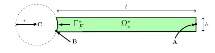
\(\Omega_s^*\) represent the initial domain, before any deformations. We denote \(\Omega^t_s\) the domain obtained during the deformations application, at the time t.
By the Newton’s second law, we can describe the fundamental equation of the solid mechanic in a Lagrangian frame. Furthermore, we will suppose that the hyperelastic material follows a compressible Saint-Venant-Kirchhoff model. The Lamé coefficients, used in this model, are deduced from the Young’s modulus \(E_s\) and the Poisson’s ratio \(\nu_s\) of the material.
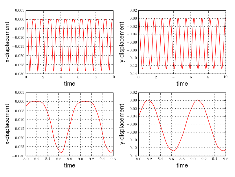
We observe, during this simulation, the displacement of \(A\), on the \(x\) and \(y\) axis, when the elastic structure is subjected to its own weight, and compare our results to the reference ones given Turek and Hron.
In the first two cases, CSM1 and CSM2, we want to determine the steady state condition. To find it, a quasi-static algorithm is used, which increase at each step the gravity parameter.
For the third cases, CSM3, we realise a transient simulation, where we will observe the comportment of \(A\) subjected to its weight during a given time span.
1.1. Boundary conditions
We set
-
on \(\Gamma_{F}^*\), a condition that imposes this boundary to be fixed : \(\boldsymbol{\eta}_s=0\)
-
on \(\Gamma_{L}^*\), a condition that lets these boundaries be free from constraints : \((\boldsymbol{F}_s\boldsymbol{\Sigma}_s)\boldsymbol{ n }^*_s=\boldsymbol{0}\)
where \(\boldsymbol{n}_s^*\) is the outer unit normal vector from \(\partial \Omega_s^*\).
1.2. Initial conditions
The source term \(\boldsymbol{f}_s\), chosen in order to set in motion the elastic structure, is define by
where \(g\) is a gravitational constant.
The reference document [TurekHron] doesn’t specify the time interval used to obtain their results. In our case, it’s chosen as \(\lbrack0,10\rbrack\).
2. Inputs
The following table displays the various fixed and variables parameters of this test-case.
| Name | Description | Nominal Value | Units |
|---|---|---|---|
\(g\) |
gravitational constant |
2 |
\(m / s^2\) |
\(l\) |
elastic structure length |
\(0.35\) |
\(m\) |
\(h\) |
elastic structure height |
\(0.02\) |
\(m\) |
\(r\) |
cylinder radius |
\(0.05\) |
\(m\) |
\(C\) |
cylinder center coordinates |
\((0.2,0.2)\) |
\(m\) |
\(A\) |
control point coordinates |
\((0.2,0.2)\) |
\(m\) |
\(B\) |
point coordinates |
\((0.15,0.2)\) |
\(m\) |
\(E_s\) |
Young’s modulus |
\(1.4\times 10^6\) |
\(kg / ms^2\) |
\(\nu_s\) |
Poisson’s ratio |
\(0.4\) |
dimensionless |
\(\rho^*_s\) |
density |
\(1000\) |
\(kg/ m^3\) |
As for solvers we used, Newton’s method is chosen for the non-linear part and a direct method based on LU decomposition is selected for the linear part.
3. Outputs
As described before, we have
We search the displacement \(\boldsymbol{\eta}_s\), on \(\Omega_s^*\), which will satisfy this equation.
In particular, the displacement of the point \(A\) is the one that interests us.
4. Discretization
To realize these tests, we made the choice to used Finite Elements Method, with Lagrangian elements of order \(N\) to discretize space.
Newmark-beta method, presented into [Chabannes] papers, is the one we used for the time discretization. We used this method with \(\gamma=0.5\) and \(\beta=0.25\).
4.1. Solvers
Here are the different solvers ( linear and non-linear ) used during results acquisition.
type |
gmres |
relative tolerance |
1e-13 |
max iteration |
1000 |
reuse preconditioner |
true |
relative tolerance |
1e-8 |
steps tolerance |
1e-8 |
max iteration |
500 |
max iteration with reuse |
10 |
reuse jacobian |
false |
reuse jacobian rebuild at first Newton step |
true |
relative tolerance |
1e-5 |
max iteration |
500 |
reuse preconditioner |
CSM1/CSM2 : false | CSM3 : true |
reuse preconditioner rebuild at first Newton step |
true |
type |
lu |
package |
mumps |
5. Implementation
To realize the acquisition of the benchmark results, code files contained and using the Feel++ library will be used. Here is a quick look to the different location of them.
First at all, the main code can be found in
feelpp/applications/models/solid
The configuration file for the CSM3 case, the only one we work on, is located at
feelpp/applications/models/solid/TurekHron
The result files are then stored by default in
feel/applications/models/solid/TurekHron/csm3/"OrderDisp""Geometric_order"/"processor_used"
Like that, for the CSM3 case executed on 8 processors, with a \(P_1\) displacement approximation space and a geometric order of 1, the path is
feel/applications/models/solid/TurekHron/csm3/P1G1/np_8
At least, to retrieve results that interested us for the benchmark and to generate graphs, we use a Python script located at
feelpp-benchmarking-book/CFD/Turek-Hron/postprocess_cfd.py
6. Results
6.1. CSM1
\(N_{elt}\) |
\(N_{dof}\) |
\(x\) displacement \(\lbrack\times 10^{-3}\rbrack\) |
\(y\) displacement \(\lbrack\times 10^{-3}\rbrack\) |
Reference [TurekHron] |
-7.187 |
-66.10 |
|
1061 |
4620 (\(P_2\)) |
-7.039 |
-65.32 |
4199 |
17540 (\(P_2\)) |
-7.047 |
-65.37 |
16495 |
67464 (\(P_2\)) |
-7.048 |
-65.37 |
1061 |
10112 (\(P_3\)) |
-7.046 |
-65.36 |
1906 |
17900 (\(P_3\)) |
-7.049 |
-65.37 |
1061 |
17726 (\(P_4\)) |
-7.048 |
-65.37 |
All the files used for this case can be found in this rep [ geo file, config file, json file ]
6.2. CSM2
\(N_{elt}\) |
\(N_{dof}\) |
\(x\) displacement \(\lbrack\times 10^{-3}\rbrack\) |
\(y\) displacement \(\lbrack\times 10^{-3}\rbrack\) |
Reference [TurekHron] |
-0.4690 |
-16.97 |
|
1061 |
4620 (\(P_2\)) |
-0.459 |
-16.77 |
4201 |
17548 (\(P_2\)) |
-0.459 |
-16.77 |
16495 |
67464 (\(P_2\)) |
-0.459 |
-16.78 |
1061 |
10112 (\(P_3\)) |
-0.4594 |
-16.78 |
16475 |
150500 (\(P_3\)) |
-0.460 |
-16.78 |
1061 |
17726 (\(P_4\)) |
-0.460 |
-16.78 |
All the files used for this case can be found in this rep [geo file, config file, json file].
6.3. CSM3
The results of the CSM3 benchmark are detailed below.
\(\Delta t\) |
\(N_{elt}\) |
\(N_{dof}\) |
\(x\) displacement \(\lbrack\times 10^{-3}\rbrack\) |
\(y\) displacement \(\lbrack\times 10^{-3}\rbrack\) |
/ |
Reference [TurekHron] |
−14.305 ± 14.305 [1.0995] |
−63.607 ± 65.160 [1.0995] |
|
0.02 |
4199 |
17536(\(P_2\)) |
-14.585 ± 14.590 [1.0953] |
-63.981 ± 65.521 [1.0930] |
4199 |
38900(\(P_3\)) |
-14.589 ± 14.594 [1.0953] |
-63.998 ± 65.522 [1.0930] |
|
1043 |
17536(\(P_4\)) |
-14.591 ± 14.596 [1.0953] |
-64.009 ± 65.521 [1.0930] |
|
4199 |
68662(\(P_4\)) |
-14.590 ± 14.595 [1.0953] |
-64.003 ± 65.522 [1.0930] |
0.01 |
4199 |
17536(\(P_2\)) |
-14.636 ± 14.640 [1.0969] |
-63.937 ± 65.761 [1.0945] |
4199 |
38900(\(P_3\)) |
-14.642 ± 14.646 [1.0969] |
-63.949 ± 65.771 [1.0945] |
|
1043 |
17536(\(P_4\)) |
-14.645 ± 14.649 [1.0961] |
-63.955 ± 65.778 [1.0945] |
|
4199 |
68662(\(P_4\)) |
-14.627 ± 14.629 [1.0947] |
-63.916 ± 65.739 [1.0947] |
0.005 |
4199 |
17536(\(P_2\)) |
-14.645 ± 14.645 [1.0966] |
-64.083 ± 65.521 [1.0951] |
4199 |
38900(\(P_3\)) |
-14.649 ± 14.650 [1.0966] |
-64.092 ± 65.637 [1.0951] |
|
1043 |
17536(\(P_4\)) |
-14.652 ± 14.653 [1.0966] |
-64.099 ± 65.645 [1.0951] |
|
4199 |
68662(\(P_4\)) |
-14.650 ± 14.651 [1.0966] |
-64.095 ± 65.640 [1.0951] |
All the files used for this case can be found in this rep [ geo file, config file, json file ]
6.4. Conclusion
To obtain these data, we used several different mesh refinements and different polynomial approximations for the displacement on the time interval \(\lbrack 0,10 \rbrack\).
Our results are pretty similar to those from Turek and Hron, despite a small gap. This gap can be caused by the difference between our time interval and the one used for the reference acquisitions.
7. Bibliography
-
[TurekHron] S. Turek and J. Hron, Proposal for numerical benchmarking of fluid-structure interaction between an elastic object and laminar incompressible flow, Lecture Notes in Computational Science and Engineering, 2006.
-
[Chabannes] Vincent Chabannes, Vers la simulation numérique des écoulements sanguins, Équations aux dérivées partielles [math.AP], Université de Grenoble, 2013.