.pdf
.pdf
ElectroMagnet
In this example, we will estimate the rise in temperature due to Joules losses in a stranded conductor. An electrical potential \(V_D\) is applied to the entry/exit of the conductor which is also water cooled.
1. Running the case
The command line to run this case in linear is
mpirun -np 4 feelpp_toolbox_thermoelectric --case "github:{path:toolboxes/thermoelectric/ElectroMagnets/HL-31_H1}"The command line to run this case in non linear is
mpirun -np 4 feelpp_toolbox_thermoelectric --case "github:{path:toolboxes/thermoelectric/ElectroMagnets/HL-31_H1}" --case.config-file HL-31_H1_nonlinear.cfg3. Geometry
The conductor consists in a solenoid, which is one helix of a magnet.
The mesh can be retrieve from girder with the following ID: 5af59e88b0e9574027047fc0 (see girder).
4. Input parameters
| Name | Description | Value | Unit | |
|---|---|---|---|---|
\(\sigma_0\) |
electric potential at reference temperature |
53e3 |
\(S/mm\) |
|
\(V_D\) |
electrical potential |
9 |
\(V\) |
|
\(\alpha\) |
temperature coefficient |
3.6e-3 |
\(K^{-1}\) |
|
L |
Lorentz number |
2.47e-8 |
\(W\cdot\Omega\cdot K^{-2}\) |
|
\(T_0\) |
reference temperature |
290 |
\(K\) |
|
h |
transfer coefficient |
0.085 |
\(W\cdot m^{-2}\cdot K^{-1}\) |
|
\(T_w\) |
water temperature |
290 |
\(K\) |
"Parameters":
{
    "sigma0":53e3, //[ S/mm ]
    "T0":290, //[ K ]
    "alpha":3.6e-3, //[ 1/K ]
    "Lorentz":2.47e-8, //[ W*Omega/(K*K) ]
    "h": "0.085", //[ W/(mm^2*K) ]
    "Tw": "290", //[ K ]
    "VD": "9" //[ V ]
},
4.1. Model & Toolbox
-
This problem is fully described by a Thermo-Electric model, namely a poisson equation for the electrical potential \(V\) and a standard heat equation for the temperature field \(T\) with Joules losses as a source term. Due to the dependence of the thermic and electric conductivities to the temperature, the problem is non linear. We can describe the conductivities with the following laws:
"k":"sigma0*Lorentz*heat_T/(1+alpha*(heat_T-T0)):sigma0:alpha:T0:Lorentz:heat_T", //[ W/(mm*K) ]
"sigma":"sigma0/(1+alpha*(heat_T-T0))+0*heat_T:sigma0:alpha:T0:heat_T"// [S/mm ]-
toolbox: thermoelectric
4.2. Materials
| Name | Description | Marker | Value | Unit | |
|---|---|---|---|---|---|
\(\sigma_0\) |
electric conductivity |
Cu |
53e3 |
\(S.m^{-1}\) |
4.3. Boundary conditions
The boundary conditions for the electrical probleme are introduced as simple Dirichlet boundary conditions for the electric potential on the entry/exit of the conductor. For the remaining faces, as no current is flowing througth these faces, we add Homogeneous Neumann conditions.
| Marker | Type | Value | |
|---|---|---|---|
V0 |
Dirichlet |
0 |
|
V1 |
Dirichlet |
\(V_D\) |
|
Rint, Rext, Interface, GR_1_Interface |
Neumann |
0 |
"electric-potential":
{
    "Dirichlet":
    {
        "V0":
        {
            "expr":"0" // V_0 [ V ]
        },
        "V1":
        {
            "expr":"VD:VD"
        }
    }
}
As for the heat equation, the forced water cooling is modeled by robin boundary condition with \(T_w\) the temperature of the coolant and \(h\) an heat exchange coefficient.
| Marker | Type | Value | |
|---|---|---|---|
Rint, Rext |
Robin |
\(h(T-T_w)\) |
|
V0, V1, Interface, GR_1_Interface |
Neumann |
0 |
"temperature":
{
    "Robin":
    {
        "Rint":
        {
            "expr1":"h:h",
            "expr2":"Tw:Tw"
        },
        "Rext":
        {
            "expr1":"h:h",
            "expr2":"Tw:Tw"
        }
    },
5. Outputs
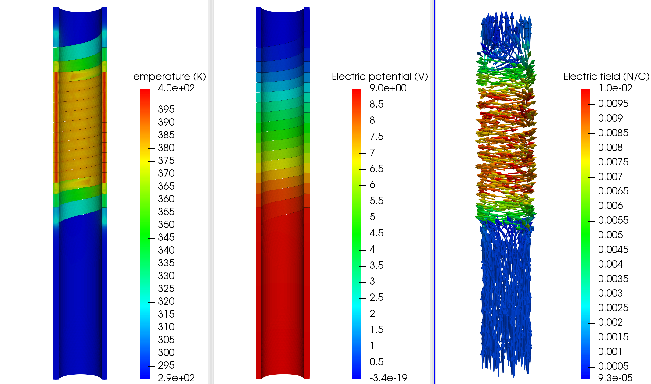
The main fields of concern are the electric potential \(V\), the temperature \(T\) and the current density \(\mathbf{j}\) or the electric field \(\mathbf{E}\) presented in the following figure.
"PostProcess":
{
    "use-model-name":1,
    "thermo-electric":
    {
        "Exports":
        {
            "fields":["heat.temperature","electric.electric-potential","electric.electric-field","electric.current-density","heat.pid"]
        }
    }
}