 .pdf
.pdf
Stokes flow in a pipe
1. Running the model
The command line to run this pipestokes case
mpirun -np 4 feelpp_toolbox_fluid --case "github:{repo:toolbox,path:examples/modules/cfd/examples/pipestokes/case_original}"Some useful commande lines:
-To edit the mesh step we must add
--gmsh.hsize=
-To edit other parameter in the geo file ( height for exemple) we must add
--fluid.gmsh.geo-variables-list="height="
-To edit json parameters we must add
--json-editions Parameters.height:n
2. Data files
2.1. Json file
2.1.1. Names and Type of Model
A model JSON file starts by giving names (long and short) as well as the type of model which will be used by the toolbox. The latter allows to configure the set of equations associated the toolbox physics.
"Name": "Stokes flow in a pipe", (1)
"ShortName":"pipestokes", (2)
"Models": (3)
{
   "equations":"Stokes" (4)
}| 1 | Name of the example, usually printed on-screen and in log files during simulations |
| 2 | Short name of the example, it is used to create directories to store the results of the simulation of the model |
| 3 | Section Models defined by the toolbox to define the main configuration of a toolbox and in particular the set of equations to be solved |
| 4 | toolbox specific option to define set of equations to be solved, read the toolbox manual to learn about the possible options. |
2.1.2. Parameters
This section of the Model JSON file defines the parameters that may enter expressions used in the subsequent sections.
Parameters section"Parameters": (1)
{
"ubar":"1.0", (2)
"height":"1.0", (3)
"vmax":"1.0",(4)
}| 1 | name of the section |
| 2 | defines a new parameter ubar and its associated value |
| 3 | define the height of the geometry |
| 4 | define the maximal velocity |
2.1.3. Materials
This section of the Model JSON file defines material properties linking the Physical Entities in the mesh data structures to these properties.
"Materials":
    {
        "Fluid": (1)
        {
            "rho":"1.0", (2)
            "mu":"1.0" (3)
        }
}| 1 | gives the name of the physical entity (here Physical Surface) associated to the Material. |
| 2 | density \(\rho\) is called rho and is given in SI units, in the stocks model there is no rho, but in the implementation of stoks equations it isused so we have to choose rho=1 in this case. |
| 3 | viscosity \(\mu\) is called mu and is given in SI units |
2.1.4. Boundary Conditions
This section of the Model JSON file defines the boundary conditions.
BoundaryConditions section"BoundaryConditions":
{
"velocity": (1)
{
"Dirichlet": (2)
{
"inlet": (3)
{
"expr":"{(vmax/(height-(height/2.))*(height/2.))*y*(height-y),0}:y:height:vmax" (4)
},
"wall1": (5)
{
"expr":"{0,0}" (6)
},
"wall2": (7)
{
"expr":"{0,0}" (8)
}
}
},
"fluid": (9)
{
"outlet": (10)
{
"outlet": (11)
{
"expr":"0" (12)
}
}
}
}| 1 | the field name of the toolbox to which the boundary condition is associated |
| 2 | the type of boundary condition to apply, here Dirichlet |
| 3 | the physical entity (associated to the mesh) to which the condition is applied |
| 4 | the mathematical expression associated to the condition |
| 5 | another physical entity to which Dirichlet conditions are applied |
| 6 | the associated expression to the entity |
| 7 | another physical entity to which Dirichlet conditions are applied |
| 8 | the associated expression to the entity |
| 9 | the variable toolbox to which the condition is applied, here fluid which corresponds to velocity and pressure \((\mathbf{u},p)\) |
| 10 | the type of boundary condition applied, here outlet or outflow boundary condition |
| 11 | the hysical entity to which outflow condition is applied |
| 12 | the expression associated to the outflow condition, note that it is scalar and corresponds in this case to the condition \(\sigma(\mathbf{u},p).n=0\) |
"PostProcess": (1)
    {
        "Exports": (2)
        {
            "fields":["velocity","pressure","pid"] (3)
        },

    }
| 1 | the name of the section |
| 2 | the Exports identifies the toolbox fields that have to be exported for visualisation |
| 3 | the list of fields to be exported |
2.2. CFG file
The Model CFG (.cfg) files allow to pass command line options to Feel++ applications. In particular, it allows to
-
setup the mesh
-
define the solution strategy and configure the linear/non-linear algebraic solvers.
The Cfg file used in this benchmark
directory=pipestokes  (1)
case.dimension=2 (2)
[fluid] (3)
filename=$cfgdir/pipestokes.json (4)
mesh.filename=$cfgdir/pipestokes.geo (5)
gmsh.hsize=0.1 (6)
pc-type=lu #gasm,lu (7)
| 1 | the directory where the results are exported |
| 2 | the dimension of the application, by default 3D |
| 3 | toolboxe prefix |
| 4 | the associated Json file |
| 5 | the geometric file |
| 6 | the mesh step |
| 7 | the chosen method for decomposition |
We didn’t configure the solver, cause in this case, the systeme is linear, and by default the solver chosen is the linear one.
3. Geometry & Input parameters
3.1. Model & Toolbox
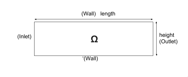
We consider a 2D model representative of a pipe, the flow domain is the rectangle \( \lbrack 0,length \rbrack \times \lbrack 0,height \rbrack \) and is characterized by its dynamic viscosity \(\mu\). we chose for this case the Stokes model.
We remind the Stokes model:
with \(\boldsymbol{\mu}\) is the dynamic viscosity, \(p\) is the pressure, \(\boldsymbol{f}\) the source term and \(\boldsymbol{u}\) the velocity field.
3.2. Initial conditions
-
Since we are not considering the time evolution in this case, we have \(v_{inlet}\) = \(D\) \(y(height-y)\). To determine \(D\), we use the fact that for \(y=\frac{height}{2}\) we have the maximal velocity, so
-
In this case, there is no source term so, \(\boldsymbol{f}=\boldsymbol{0}\).
3.3. Boundary conditions
-
On wall, a homogenous Dirichlet condition \(\boldsymbol{u}=\boldsymbol{0}\)
-
On outlet, a Neumann condition \(\boldsymbol{\sigma} . \boldsymbol{n}=0\), where \(\boldsymbol{\sigma}=-p\boldsymbol{I}_d+2\mu\boldsymbol{D}(\boldsymbol{u})\) and \(\boldsymbol{D}(\boldsymbol{u})=\frac{1}{2}(\nabla \boldsymbol{u}+\nabla \boldsymbol{u}^{T})\), \(\boldsymbol{\sigma} \) is the contraint tensor and \(\boldsymbol{D}\) is the deformation tensor.
-
On inlet, an inflow Dirichlet condition : \( \boldsymbol{u}=(v_{inlet},0) \)
4. Benchmark
4.1. Results
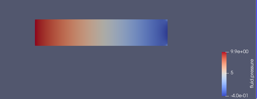
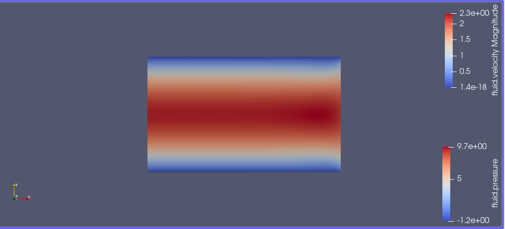
We find the Results in "/feel/pipestokes/np_1/fluid.exports", if we want to show the figure using Paraview we have to use the file Export.case Using height=1, lenght=5 and vmax=1 we found thoses figures
-
For the pressure
-
For the velocity
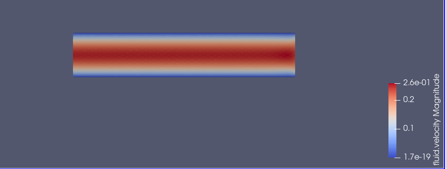
we can also show the arrows to see the direction of the flow, the figure below that the directions is from the left to the right, which means that the theory expectation are verified, I mean by the theory expectation that the flow of blood must go from the highest pression to the lowest.
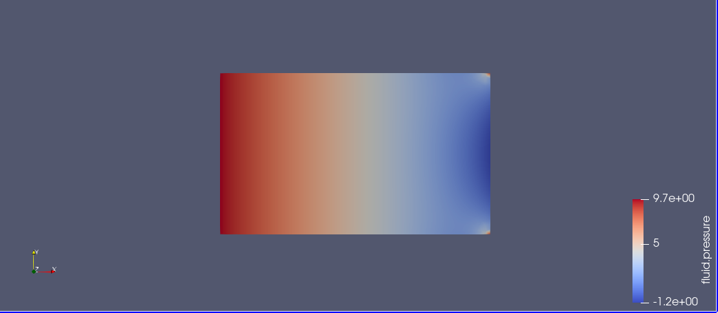
Using height=3, lenght=5 and vmax=1, to change it we can use
feelpp_toolbox_fluid --case "github:{repo:toolbox,path:examples/modules/cfd/examples/pipestokes}" --fluid.gmsh.geo-variables-list="height=3" --json-editions Parameters.height:3
-
For the pressure
-
For the velocity
4.2. Issues
We notice in the case above, the presence of two white points on the top of the outlet, we can also see the deflection of the arrows in the figure above. which is not normal, the probleme is in the bondary conditions, precisly the outlet one. besides,we added the calculation of the error in the file json
Three solutions were suggested by PRUD’HOMME and CHABANNES
4.2.1. First case
Instead of putting \(\sigma.n=0\), We calculate the expression of \(\sigma\) and put the exact expression.
The command line to run this case is
mpirun -np 4 feelpp_toolbox_fluid --case "github:{repo:toolbox,path:examples/modules/cfd/examples/pipestokes/case_corrections/naumann}"We already know the expression of \(u=Dy(1-y)\), and we know that the pression p is linear so \(p=ax+b\).
The first equation of stokes give us that \(f=-\mu\Delta u+\nabla p\), we have \(\nabla p=(a,0)\) and \(\Delta u=(-2D,0)\).
so \(f=(2\mu D+a,0)\), in our case we had no external force (\(f=0\)), to respect that, we have to choose a=-2\mu D.
To detect the expression of b, we assumed that the pressure has a zero average, it means that
[stem]:
So \(b*lenght=height* \mu D*lenght^{2}\), b=\(heigh \mu D*lenght\)
The expression of p is p=-2 \(\mu Dx+height*\mu *D* lenght\).
We know that \(\sigma.n=-pI_{d}+2\mu D(u)\) we calculate D(u)
So
On as
So
That’s means that
For the data files the cfg didn’t change, we changed just the boundary conditions in the json, precisely the outlet condition.
4.2.2. Second case
We put Dirichlet conditions everywhere, we know that the velocity is quadratic, so the velocity in outlet is the same that the one in inlet.
The command line to run this case is
mpirun -np 4 feelpp_toolbox_fluid --case "github:{repo:toolbox,path:examples/modules/cfd/examples/pipestokes/case_corrections/dirichlet}"The data files for this case
4.2.3. Third case
We fixe that the tengential velocity is null and we fixe a value for p.
The command line to run this case is
mpirun -np 4 feelpp_toolbox_fluid --case "github:{repo:toolbox,path:examples/modules/cfd/examples/pipestokes/case_corrections/pression}"The data files for this case
4.2.4. Error
To calculate the error, I add this part in the json file (based on the documentation of CHABANNES).
    "PostProcess":
    {
          "Measures":
        {

             "Norm":
             {
               "mynorm": (1)
               {
                 "type":"L2", (2)
                 "field":"velocity" (3)
               },
              "myerror": (4)
              {
                "type":"L2-error", (5)
                "field":"velocity", (6)
                "solution":"{(vmax/((height-(height/2.))*(height/2.)))*y*(height-y),0}:y:height:vmax" (7)
              }
            }
        }
    }
| 1 | the name associated with the first norm computation |
| 2 | the norm type |
| 3 | the field u evaluated in the norm (here the velocity field in the fluid toolbox) |
| 4 | the name associated with the second norm computation |
| 5 | the norm type |
| 6 | the field u evaluated in the norm |
| 7 | the expression v with the error norm type |
The results are stored in a CSV file at columns named Norm_mynorm_L2 and Norm_myerror_L2-error.
Results:
| cases | Norm_mynorm_L2 | Norm_myerror_L2-error |
|---|---|---|
|
1.6329931618554512e+00 |
3.3760622864791791e-15 |
|
1.6329931618555187e+00 |
2.0511969262388929e-11 |
|
1.6329931618554521e+00 |
3.7887047021696832e-15 |
4.3. Comparison
We saw that in CFG file, we can choose between two decomposition LU and Gasm, in the theory, the option Gasm is faster than LU, in fact Gasm decompose the domaine and it use LU in every part in parallel.
We decide to refine the mesh and compare the run time for both options.
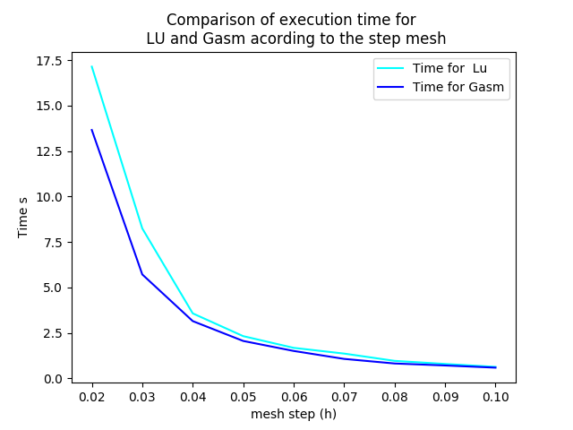
we notice that the execution time decreases for both options, when the mesh step becomes coarse, which coincides with the theoretical results. And we can see also that the curve corresponds to the Gasm method is faster.
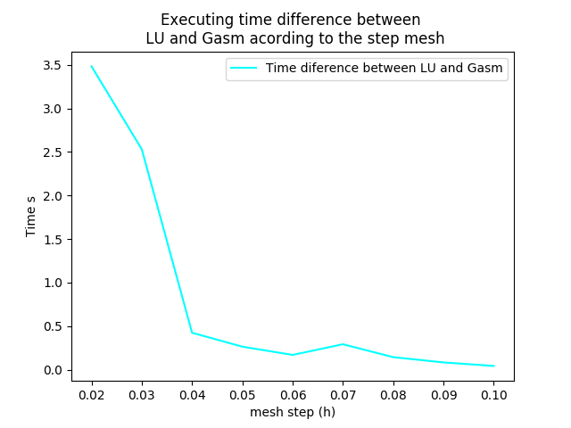
The curve above corresponds to the time difference between the two methods, we can see that when the mesh step is large, the time differance is really small, on the other hand the time differance is big when the step mesh is small.