Turek-Hron FSI Benchmark

In order to validate our fluid-structure interaction solver, a benchmark, initially proposed by [TurekHron], is realized.

Computer codes, used for the acquisition of results, are from [Chabannes].

Note: This benchmark is linked to the Turek-Hron CFD and Turek-Hron CSM benchmarks.

1. Problem Description

In this case, we want to study the flow of a laminar incrompressible flow around an elastic obstacle, fixed to a rigid cylinder. The geometry is given with Figure Geometry of the Turek & Hron FSI Benchmark.. We denote \(\Omega_f^*\) the fluid domain, represented by a rectangle of dimension \( [0,2.5] \times [0,0.41] \). This domain is characterized by its density \(\rho_f\) and its dynamic viscosity \(\mu_f\). In this case, the fluid material we used is glycerin.

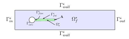
Figure 1 : Geometry of the Turek & Hron FSI Benchmark.

The model chosen to describe the flow is the incompressible Navier-Stockes model. On the other side, the structure domain, named \(\Omega_s^*\), is described by a hyperelastic equation with Saint-Venant-Kirchhoff law.

2. Inputs

The following table displays the various fixed and variables parameters of this test-case.

Table 1. Fixed and Variable Input Parameters
Name	Description	Nominal Value	Units
\(l\)	elastic structure length	\(0.35\)	\(m\)
\(h\)	elastic structure height	\(0.02\)	\(m\)
\(r\)	cylinder radius	\(0.05\)	\(m\)
\(C\)	cylinder center coordinates	\((0.2,0.2)\)	\(m\)
\(A\)	control point coordinates	\((0.2,0.2)\)	\(m\)
\(B\)	point coordinates	\((0.15,0.2)\)	\(m\)
\(E_s\)	Young’s modulus	\(5.6 \times 10^6\)	\(kg.m^{-1}s^{-2}\)
\(\nu_s\)	Poisson’s ratio	\(0.4\)	dimensionless
\(\rho_s\)	structure density	\(1000\)	\(kg.m^{-3}\)
\(\nu_f\)	kinematic viscosity	\(1\times 10^{-3}\)	\(m^2.s^{-1}\)
\(\mu_f\)	dynamic viscosity	\(1\)	\(kg.m^{-1}.s^{-1}\)
\(\rho_f\)	density	\(1000\)	\(kg.m^{-3}\)
\(f_f\)	source term	0
\(\bar{U}\)	mean inflow velocity	2	\(m.s^{-1}\)

2.1. Boundary conditions

We set

on \(\Gamma_{in}^*\), an inflow Dirichlet condition : \( \boldsymbol{u}_f=(v_{in},0);\)
on \(\Gamma_{wall}^* \cup \Gamma_{circ}^*\), a homogeneous Dirichlet condition : \(\boldsymbol{u}_f=\boldsymbol{0};\)
on \(\Gamma_{out}^*\), a Neumann condition : \(\boldsymbol{\sigma}_f\boldsymbol{n}_f=\boldsymbol{0};\)
on \(\Gamma_{fixe}^*\), a condition that imposes this boundary to be fixed : \(\boldsymbol{\eta}_s=0;\)
on \(\Gamma_{fsi}^*\) :

\[\frac{\partial \boldsymbol{\eta_{s}} }{\partial t} - \boldsymbol{u}_f \circ \mathcal{A}^t_f = \boldsymbol{0} \quad \left( \text{Velocities continuity}\right)\]

\[ \boldsymbol{F}_{s} \boldsymbol{\Sigma}_{s} \boldsymbol{n}^*_s + J_{\mathcal{A}^t_f} \boldsymbol{F}_{\mathcal{A}^t_f}^{-T} \hat{\boldsymbol{\sigma}}_f \boldsymbol{n}^*_f = \boldsymbol{0} \quad \left( \text{ Constraint continuity}\right)\]

\[ \boldsymbol{\varphi}_s^t - \mathcal{A}^t_f = \boldsymbol{0} \quad \left( \text{Geometric continuity}\right)\]

where \(\boldsymbol{n}_f\) is the outer unit normal vector from \(\partial \Omega_f^*\).

In order to describe the flow inlet by \(\Gamma_{in}\), a parabolic velocity profile is used. It can be expressed by

\[ v_{cst} = 1.5 \bar{U} \frac{4}{0.1681} y \left(0.41-y\right)\]

where \(\bar{U}\) is the mean inflow velocity.

However, to impose a progressive increase of this velocity profile, we define

\[ v_{in} = \left\{ \begin{aligned} & v_{cst} \frac{1-\cos\left( \frac{\pi}{2} t \right) }{2} \quad & \text{ if } t < 2 \\ & v_{cst} \quad & \text{ otherwise } \end{aligned} \right. \]

With t the time.

2.2. Initial conditions

The fluid and the solid are at rest.

3. Outputs

The quantities we observe during this benchmark are on one hand the lift and drag forces ( respectively \(F_L\) and \(F_D\) ), as well as the displacement, on \(x\) and \(y\) axis, of the point A is the second value that interest us here.

4. Discretization

To realize these tests, we made the choice to used \(P_N~-~P_{N-1}\) Taylor-Hood finite elements to discretize the fluid space. For the time discretization, we use :

a BDF at order 2 is used for the fluid
a Newmark scheme for the structure, with parameters \(\gamma=0.5\) and \(\beta=0.25\).

Theses choices are described for example in [Chabannes].

5. Results

First at all, we will discretize the simulation parameters for the different cases studied.

Table 2. Discretizations
	\(N_{elt}\)	\(N_{dof}\)	\( [P^N_c(\Omega_{f,\delta}]^2 \times P^{N-1}_c(\Omega_{f,\delta}) \times V^{N-1}_{s,\delta}\)	\(\Delta t\)
[TurekHron]	15872	304128		0.00025
(1)	1284	27400	\( [P^4_c(\Omega_{f,(h,3)}]^2 \times P^3_c(\Omega_{f,(h,3)}) \times V^3_{s,(h,3)}\)	0.005
(2)	2117	44834	\( [P^4_c(\Omega_{f,(h,3)}]^2 \times P^3_c(\Omega_{f,(h,3)}) \times V^3_{s,(h,3)}\)	0.005
(3)	4549	95427	\( [P^4_c(\Omega_{f,(h,3)}]^2 \times P^3_c(\Omega_{f,(h,3)}) \times V^3_{s,(h,3)}\)	0.005
(4)	17702	81654	\( [P^2_c(\Omega_{f,(h,1)}]^2 \times P^1_c(\Omega_{f,(h,1)}) \times V^1_{s,(h,1)}\)	0.0005

Then the FSI3 benchmark results are detailed below.

Table 3. Results for FSI3
	\(x\) displacement \( [\times 10^{-3}] \)	\(y\) displacement \( [\times 10^{-3}] \)	Drag	Lift
[TurekHron]	-2.69 ± 2.53 [10.9]	1.48 ± 34.38 [5.3]	457.3 ± 22.66 [10.9]	2.22 ± 149.78 [5.3]
[Breuer]			464.5 ± 40.50	6.00 ± 166.00 [5.5]
[TurekHron2]	-2.88 ± 2.72 [10.9]	1.47 ± 34.99 [5.5]	460.5 ± 27.74 [10.9]	2.50 ± 153.91 [5.5]
[MunschBreuer]	-4.54 ± 4.34 [10.1]	1.50 ± 42.50 [5.1]	467.5 ± 39.50 [10.1]	16.2 ± 188.70 [5.1]
[Gallinger]			474.9 ± 28.10	3.90 ± 165.90 [5.5]
[Sandboge]	-2.83 ± 2.78 [10.8]	1.35 ± 34.75 [5.4]	458.5 ± 24.00 [10.8]	2.50 ± 147.50 [5.4]
(1)	-2.86 ± 2.74 [10.9]	1.31 ± 34.71 [5.4]	459.7 ± 29.97 [10.9]	4.46 ± 172.53 [5.4]
(2)	-2.85 ± 2.72 [10.9]	1.35 ± 34.62 [5.4]	459.2 ± 29.62 [10.9]	3.53 ± 172.73 [5.4]
(3)	-2.88 ± 2.75 [10.9]	1.35 ± 34.72 [5.4]	459.3 ± 29.84 [10.9]	3.19 ± 171.20 [5.4]
(4)	-2.90 ± 2.77 [11.0]	1.33 ± 34.90 [5.5]	457.9 ± 31.79 [11.0]	8.93 ± 216.21 [5.5]

5.1. Conclusion

Our first three results are quite similar to given references values. That show us that high order approximation order for space and time give us accurate values, while allow us to use less degree of freedom.

However, the lift force seems to undergo some disturbances, compared to reference results, and it’s more noticeable in our fourth case. This phenomenon is describe by [Beuer], where they’re explaining these disturbances are caused by Aitken dynamic relaxation, used in fluid structure relation for the fixed point algorithm.

In order to correct them, they propose to lower the fixed point tolerance, but this method also lowers calculation performances. An other method to solve this deviation is to use a fixed relaxation parameter \(\theta\). In this case, the optimal \(\theta\) seems to be equal to \(0.5\).

6. Bibliography

References for this benchmark

[TurekHron] S. Turek and J. Hron, Proposal for numerical benchmarking of fluid-structure interaction between an elastic object and laminar incompressible flow, Lecture Notes in Computational Science and Engineering, 2006.
[Chabannes] Vincent Chabannes, Vers la simulation numérique des écoulements sanguins, Équations aux dérivées partielles [math.AP], Université de Grenoble, 2013.
[Breuer] M. Breuer, G. De Nayer, M. Münsch, T. Gallinger, and R. Wüchner, Fluid–structure interaction using a partitioned semi-implicit predictor–corrector coupling scheme for the application of clarge-eddy simulation, Journal of Fluids and Structures, 2012.
[TurekHron2] S. Turek, J. Hron, M. Madlik, M. Razzaq, H. Wobker, and JF Acker, Numerical simulation and benchmarking of a monolithic multigrid solver for fluid-structure interaction problems with application to hemodynamics, Fluid Structure Interaction II, pages 193–220, 2010.
[MunschBreuer] M. Münsch and M. Breuer, Numerical simulation of fluid–structure interaction using eddy–resolving schemes, Fluid Structure Interaction II, pages 221–253, 2010.
[Gallinger] T.G. Gallinger, Effiziente Algorithmen zur partitionierten Lösung stark gekoppelter Probleme der Fluid-Struktur-Wechselwirkung, Shaker, 2010.
[Sandboge] R. Sandboge, Fluid-structure interaction with openfsitm and md nastrantm structural solver, Ann Arbor, 1001 :48105, 2010.