 .pdf
.pdf
Inflatable box
We will provide a 2D example of fluid-structure interaction taken from the articles
-
Küttler, U., Förster, C. & Wall, W.A. Comput Mech (2006) 38: 417. doi.org/10.1007/s00466-006-0066-5
-
A.E.J. Bogaers, S. Kok, B.D. Reddy, T. Franz, "Extending the robustness and efficiency of artificial compressibility for partitioned fluid-structure interactions", doi.org/10.1016/j.cma.2014.08.021
1. Introduction
We will simulate the inflation of a deformable box under continuous immission of an incompressible fluid. The structure is made of one solid elastic rectangular shell which is filled through an opening.
In this model, fluid’s boundary conditions are only of Dirichlet type. It is known that this situation is difficult to be tackled using partitioned solvers with Dirichlet-Neumann discretization of FSI coupling conditions. There are two reasons for this: the so called incompressiblity condition dilemma, and the fact that pressure’s absolute value is not known. The incompressibility condition dilemma can be described as follows: whenever the structure’s displacement is calculated, it should take into account the fluid’s volume change in the next time step to be admissible and produce an admissible interface velocity (compatible with incompressibility condition inside the fluid subdomain). In a Dirichlet-Neumann approach, this is not the case: in fact, the new interface, computed with Neumann conditions on the solid subproblem, and the new interface velocity computed through finite differences do not, a priori, satisfy such constraint. The pressure issue, finally, can be solved by prescribing a pressure value on the boundary of the fluid domain. We will perform the simulation applying a Generalized Robin-Neumann coupling condition, which will avoid these problems.
2. Model/Geometry
The numerical domain is shown in the figure below. We will indicate by \(\Omega_f^*\) and \(\Omega_s^*\) the initial fluid and solid subdomain, respectively.
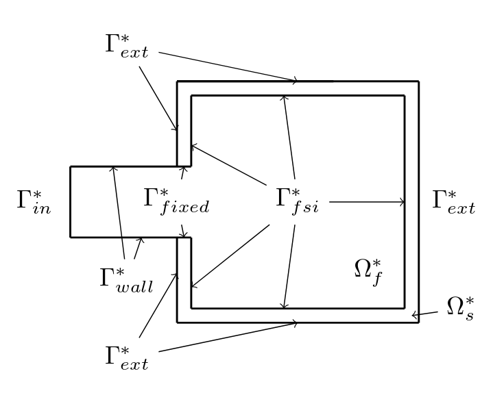
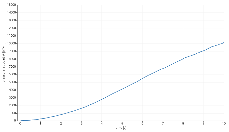
The outer box is \(3.4 m\) large, the shell is \(0.2 m\) thick, the inlet is \(1 m\) wide and positioned at \(2 m\) from the left side of the box. We will measure the pressure at point A, the mid point of the inlet upper wall.
3. Materials and Boundary Conditions
We employ materials having the following properties:
| Name | Description | Nominal Value | Units |
|---|---|---|---|
\(E\) |
Young modulus |
\(7 \cdot 10^5\) |
\(kg/m^2\) |
\(\nu\) |
Poisson coefficient |
\(0.45\) |
|
\(\rho_s\) |
Density |
\(10^3\) |
\(kg/m^3\) |
| Name | Description | Nominal Value | Units |
|---|---|---|---|
\( \mu_f \) |
Dynamic viscosity |
\(0.1606\) |
\(kg/(ms)\) |
\(\rho_f\) |
Density |
\(1.1\) |
\(kg/m^3\) |
We will use a Neo-Hookean hyperelastic model for the structure and a Newtonian stress tensor for the fluid.
We impose the following boundary conditions on the domain:
-
on \(\Gamma_{in}^*\), an inflow parabolic Dirichlet condition on fluid velocity;
-
on \(\Gamma_{wall}^*\), a homogeneous Dirichlet condition on fluid velocity : \(\boldsymbol{u}_f = \boldsymbol{0}\);
-
on \(\Gamma_{ext}^*\), a homogeneous Neumann condition on solid forces \(\boldsymbol{\sigma}_s = \boldsymbol{0}\);
-
on \(\Gamma_{fixed}^*\), a zero displacement condition on the solid side \(\boldsymbol{\eta}_s = \boldsymbol{0}\) and a homogeneous Dirichlet condition on the fluid side;
-
on \(\Gamma_{fsi}^*\) :
where \(\boldsymbol{n}_f\) is the outer unit normal vector from \(\partial \Omega_f^*\).
The inflow parabolic profile is imposed progressively: up to time \(t=1\) it is multiplied by \(\sin(\frac{\pi t}{2})\).
4. Results
We have used a structured mesh to obtain the results that we present: in the first figure we show the pressure value that was measured at point A
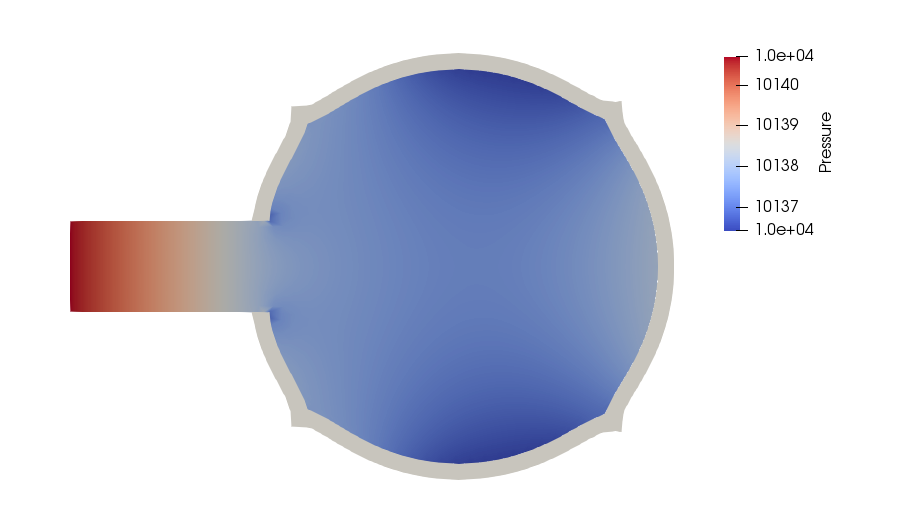
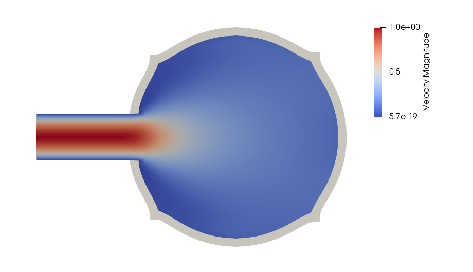
and in the following we show the profiles of pressure and velocity modulus, which qualitatively agree with those presented in the reference articles.
5. Methodology
These results were obtained by using the Feel++ 2D Fluid Structure Interaction application. The simulation was run on 24 processors using the following command:
$ mpirun -np 24 /usr/local/bin/feelpp_toolbox_fsi_2d --config-file box-balloon.cfgThe information regarding material properties and boundary conditions were specified in .json files, the geometry in the .geo file and the numerical specifications characterizing the simulation (solvers, preconditioners, constitutive models, …) in the .cfg file. The material parameters are specified as follows:
    "Materials":
    {
        "Fluid": {
            "rho":"1.1",
            "mu":"0.1606"
        }
    },
"Materials":
{
"Solid": {
"E":"7e5",
"nu":"0.45",
"rho":"1e3"
}
},The boundary conditions, instead, are specified in the following manner:
    "BoundaryConditions":
    {
        "velocity":
        {
            "Dirichlet":
            {
                "wall":
                {
                    "expr":"{0,0}"
		},
		"fixed":
		{
		"expr":"{0,0}" // necessary ??
		}
            },
            "interface_fsi":
            {
                "fsi":
                {
                    "expr":"0"
                }
            }
	},
	"fluid":
	{
	    "inlet":
	    {
		"inlet":
		{
		    "shape":"parabolic",
		    "constraint":"velocity_max",
		    "expr":"sin(pi*t/2)*(t<1)+(1-(t<1)):t"
		}
	    }
        }
    },
"BoundaryConditions":
{
"displacement":
{
"Dirichlet":
{
"fixed":
{
"expr":"{0,0}"
}
},
"interface_fsi":
{
"fsi":
{
"expr":"0"
}
},
"Neumann_scalar":
{
"free-solid":
{
"expr":"0"
}
}
}
},