 .pdf
.pdf
Lid-driven Cavity Flow benchmark
This test case has originally been proposed by [MokWall].
Computer codes, used for the acquisition of results, are from Vincent [Chabannes].
This benchmark has aso been realized by [Gerbeau], [Vàzquez], [Kuttler] and [Kassiotis].
1. Problem Description
We study here an incompressible fluid flowing into a cavity, where its walls are elastic. We use the following geometry to represent it.
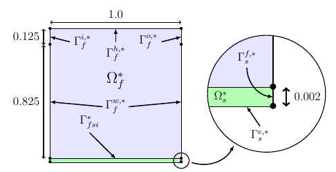
The domain \(\Omega_f^*\) is define by a square \( [0,1]^2 \), \(\Gamma^{i,*}_f\) and \(\Gamma^{o,*}_f\) are respectively the flow entrance and the flow outlet. A constant flow velocity, following the \(x\) axis, will be imposed on \(\Gamma_f^{h,*}\) border, while a null flow velocity will be imposed on \(\Gamma_f^{f,*}\). This last point represent also a non-slip condition for the fluid.
Furthermore, we add a structure domain, at the bottom of the fluid one, named \(\Omega_s^*\). It is fixed by his two vertical sides \(\Gamma_s^{f,*}\), and we denote by \(\Gamma_f^{w,*}\) the border which will interact with \(\Omega_f^*\).
During this test, we will observe the displacement of a point \(A\), positioned at \((0;0.5)\), into the \(y\) direction, and compare our results to ones found in other references.
1.1. Boundary conditions
Before enunciate the boundary conditions, we need to describe a oscillatory velocity, following the x axis and dependent of time.
Then we can set
-
on \(\Gamma^{h,*}_f\), an inflow Dirichlet condition : \(\boldsymbol{u}_{f} = ( v_{in}, 0 )\)
-
on \(\Gamma^{i,*}_f\), an inflow Dirichlet condition : \(\boldsymbol{u}_{f} = ( v_{in}(8 y -7) ,0)\)
-
on \(\Gamma^{f,*}_f\), a homogeneous Dirichlet condition : \(\boldsymbol{u}_{f} = \boldsymbol{0}\)
-
on \(\Gamma^{o,*}_f\), a Neumann condition : \(\boldsymbol{\sigma}_{f} \boldsymbol{n}_f = \boldsymbol{0}\)
-
on \(\Gamma^{f,*}_s\), a condition that imposes this boundary to be fixed : \(\boldsymbol{\eta}_{s} = \boldsymbol{0}\)
-
on \(\Gamma^{e,*}_s\), a condition that lets these boundaries be free from constraints : \(\boldsymbol{F}_{s} \boldsymbol{\Sigma}_s \boldsymbol{n}_s = \boldsymbol{0}\)
To them we also add the fluid-structure coupling conditions on \(\Gamma_{fsi}^*\) :
2. Inputs
The following table displays the various fixed and variables parameters of this test-case.
Name |
Description |
Nominal Value |
Units |
\(E_s\) |
Young’s modulus |
\(250\) |
\(N.m^{-2}\) |
\(\nu_s\) |
Poisson’s ratio |
\(0\) |
dimensionless |
\(\rho_s\) |
structure density |
\(500\) |
\(kg.m^{-3}\) |
\(\mu_f\) |
viscosity |
\(1\times 10^{-3}\) |
\(m^2.s^{-1}\) |
\(\rho_f\) |
density |
\(1\) |
\(kg.m^{-3}\) |
3. Outputs
\((\boldsymbol{u}_f, p_f, \boldsymbol{\eta}_s, \mathcal{A}_f^t)\), checking the fluid-structure system, are the output of this problem.
4. Discretization
To discretize space, we used \(P_N~-~P_{N-1}\) Taylor-Hood finite elements.
For the structure time discretization, Newmark-beta method is the one we used. And for the fluid time discretization, we used BDF, at order \(q\).
5. Implementation
All the codes files are into FSI
6. Results
We begin with a \(P_2~-~P_1\) approximation for the fluid with a geometry order equals at \(1\), and a fluid-structure stable interface.
Then we retry with a \(P_3~-~P_2\) approximation for the fluid with a geometry order equals at \(2\), and a fluid-structure stable interface.
Finally we launch it with the same conditions as before, but with a deformed interface.
6.1. Conclusion
First at all, we can see that the first two tests offer us similar results, despite different orders uses. At contrary, the third result set are better than the others.
The elastic wall thinness, in the stable case, should give an important refinement on the fluid domain, and so a better fluid-structure coupling control. However, the deformed case result are closer to the stable case made measure.
7. Bibliography
-
[MokWall] DP Mok and WA Wall, Partitioned analysis schemes for the transient interaction of incompressible flows and nonlinear flexible structures, Trends in computational structural mechanics, Barcelona, 2001.
-
[Chabannes] Vincent Chabannes, Vers la simulation numérique des écoulements sanguins, Équations aux dérivées partielles [math.AP], Université de Grenoble, 2013.
-
[Gerbeau] J.F. Gerbeau, M. Vidrascu, et al, A quasi-newton algorithm based on a reduced model for fluid-structure interaction problems in blood flows, 2003.
-
[Vazquez] J.G. Valdés Vazquèz et al, Nonlinear analysis of orthotropic membrane and shell structures including fluid-structure interaction, 2007.
-
[KuttlerWall] U. Kuttler and W.A. Wall, Fixed-point fluid–structure interaction solvers with dynamic relaxation, Computational Mechanics, 2008.
-
[Kassiotis] C. Kassiotis, A. Ibrahimbegovic, R. Niekamp, and H.G. Matthies, Nonlinear fluid–structure interaction problem ,part i : implicit partitioned algorithm, nonlinear stability proof and validation examples, Computational Mechanics, 2011.