.pdf
.pdf
2D building with natural convection
In this example, we simulate the phenomena of natural convection in an apartment of 2 rooms.
We use the Navier-Stokes model to simulate the natural convection and the toolbox heatfluid to solve it.
1. Running the case
The command line to run this case is
mpirun -np 8 feelpp_toolbox_heatfluid --case "github:{repo:toolbox,path:examples/modules/heatfluid/examples/2Dbuilding_NS}"2. Data files
The case data files are available in Github here
3. Model
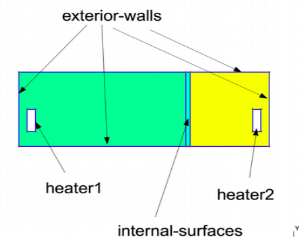
\(\quad\)The 2D thermal model of two parts separated by plaster is considered. It is an object of \(\mathbb{R}^2\), it is subdivided into different domains \(\Omega_i, i = 1,2,3\) (see the image). The sources of heat \(heater_i, i = 1,2\) are the two radiators each of which is located downstairs in each room. The heat \(T\) released in the subdomains is calculated thanks to the equation of heat transfer.
|
Boundary condition:
-
Condition of velocity
On exterior-wall, internal-surfaces, heater1, heater2
We define the vitess of zero fluid on the walls to assume that there is no circulation of flow in boundary.
-
Condition of temperature
-
Condition of Dirichlet
-
On heater1: T= 310 K
On heater2: T= 300 K
By fixing the values in two boundary heater1 and heater2, we assure the temperature for two radiators allong the simulation.
-
Condition de Robin sur exterior-wall
On the walls , we consider a wall composed of several materials (insulation / plaster / concrete) and an exchange with the outside which is at a temperature of 280 K (\(T_{ext} = 280\)).
As a a wall composed of several materials, we have to determine the heat transfer coeffient by the method which is useful to find the heat transfert between simple element such as walls in buidings, within materials. (see [1])
where
x = the wall thickness
k = the thermal conductivity of materials
h = the individual convection heat transfer coefficient for each fluid
Conditions at the interface \(\Gamma_{ij} = \Omega_i \cap \Omega_j\)
Initial condition to \(t = 0s\)
3.1. Input
| Notation | Description | Value | Unit | Note |
|---|---|---|---|---|
Paramètres globale |
||||
\(t\) |
times |
s |
||
\(T\) |
temperature |
\(K\) |
||
\(T_{ext}\) |
outside temperature |
280 |
\(K\) |
|
\(T_0\) |
initial temperature |
280 |
\(K\) |
|
\(H\) |
height |
\(1,2,3\) |
\(m\) |
|
Air |
||||
\(k\) |
thermal conductivity |
0.03 |
\(W.m^{-3}.K^{-1}\) |
|
\(\rho\) |
mass volumique |
1 |
\( kg/(m^3) \) |
|
\(Cp\) |
thermal capacity |
1004 |
\( J/(kg*K) \) |
|
\(h\) |
heat transfer coefficient |
1.0/(0.06+0.01/0.5 + 0.3/0.8 + 0.20/0.032 +0.016/0.313 +0.14) |
\( W.m^{−2}.K^{−1} \) |
|
\(\beta\) |
coefficient of thermal expansion |
0.003660 |
\(K^{-1}\) |
|
internal wall |
||||
\(k\) |
thermal conductivity |
0.25 |
\(W.m^{-3}.K^{-1}\) |
|
\(\rho\) |
mass volumique |
1 |
\( kg/(m^3) \) |
|
\(Cp\) |
thermal capacity |
1000 |
\( J/(kg*K) \) |
|
\(h\) |
heat transfer coefficient |
1.0/(0.06+0.01/0.5 + 0.3/0.8 + 0.20/0.032 +0.016/0.313 +0.14) |
\( W.m^{−2}.K^{−1} \) |
|
\(\beta\) |
coefficient of thermal expansion |
0. |
\(K^{-1}\) |
|
3.3. Implementation
directory=applications/models/aerothermics/ThermalBuilding/2d

case.dimension=2

[heat-fluid]
mesh.filename=$cfgdir/aero.geo
gmsh.hsize=0.025#0.01#0.02#0.07#0.1
filename=$cfgdir/aero.json

use-natural-convection=1
Boussinesq.ref-temperature=280#293.15

snes-monitor=1
pc-type=lu
ksp-type=preonly

[heat-fluid.heat]
initial-solution.temperature=280#293.15
bdf.order=2

[heat-fluid.fluid]
#solver=Newton #Oseen,Picard,Newton

define-pressure-cst=1
define-pressure-cst.method=algebraic#penalisation#algebraic
define-pressure-cst.markers=air1,air2

bdf.order=2

[ts]
time-step=50#10
time-final=15000
#restart=true
restart.at-last-save=true
#time-initial=0.0002
#save.freq=2
file-format=hdf5
// -*- mode: javascript -*-
{
"Name": "Thermo dynamics",
"ShortName":"ThermoDyn",
"Models":
{
"use-model-name":1,
"fluid":
{
"equations": "Navier-Stokes"
}
},
"Materials":
{
"air":
{
"markers":["air1","air2"],
"physics":["fluid","heat"],
"rho":"1",
"mu":"2.65e-2",
"k":"0.03",
"Cp":"1004",
"beta":"0.003660" //0.00006900
},
"internal-walls":
{
"markers":"internal-walls",
"physics":"heat",
//"k11":"0.02"//[ W/(m*K) ]
// //"k11":"0.0262"//[ W/(m*K) ]
// //"Cp":"1000", //[ J/(kg*K) ]
// //"rho":"150" //[ kg/(m^3) ]
"rho":"150",//820,//"82",
"k":"0.25",//"0.25",
"Cp":"1000",
"mu":"1.",//???
"beta":"0."//"0.003660"//???
}
},
"BoundaryConditions":
{
"velocity":
{
"Dirichlet":
{
"exterior-walls": { "expr":"{0,0}" },
"internal-surfaces": { "expr":"{0,0}" },
"heater1": { "expr":"{0,0}" },
"heater2": { "expr":"{0,0}" }
}
},
"temperature":
{
"Dirichlet":
{
"heater1": { "expr":"310"/*"330"*/ },
"heater2": { "expr":"300"/*"320"*/ }
},
"Robin":
{
"exterior-walls":
{
"expr1":"1.0/(0.06+0.01/0.5 + 0.3/0.8 + 0.20/0.032 +0.016/0.313 +0.14)",// h coeff
"expr2":"280"// temperature exterior
},
"exterior-walls-nofluid":
{
"expr1":"1.0/(0.06+0.01/0.5 + 0.3/0.8 + 0.20/0.032 +0.016/0.313 +0.14)",// h coeff
"expr2":"280"// temperature exterior
}
}
}
},
"PostProcess":
{
"use-model-name":1,
"heat-fluid":
{
"Exports":
{
"fields":["fluid.velocity","fluid.pressure","heat.temperature","fluid.pid"]
}
},
"fluid":
{
},
"heat":
{
}
}
}mpirun -np 16 feelpp_toolbox_heatfluid_2d --config-file aero.cfgcase with link to folder which represents a remote data in a github repository.mpirun -np 8 feelpp_toolbox_heat --case "github:{repo:toolbox,path:examples/modules/heatfluid/examples/2Dbuilding_NS}"You can also use some options to change the variables like time-final, taille du maillage hsize, …
mpirun -np 8 feelpp_toolbox_heat --case "github:{repo:toolbox,path:examples/modules/heatfluid/examples/2Dbuilding_NS}" --ts.time-final 30003.4. Result
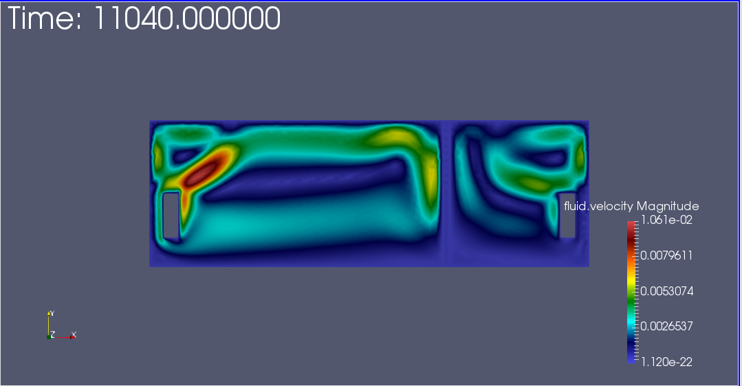
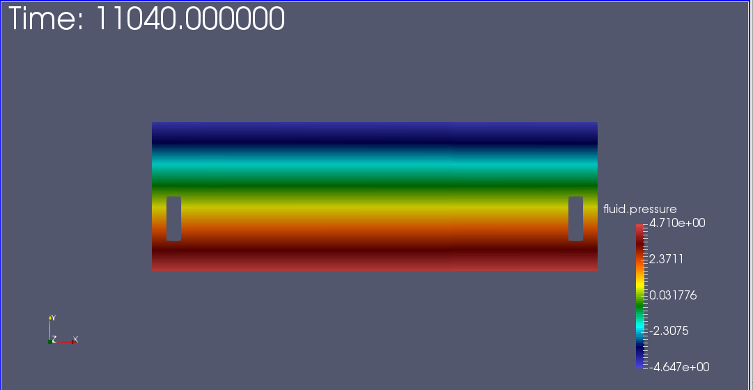
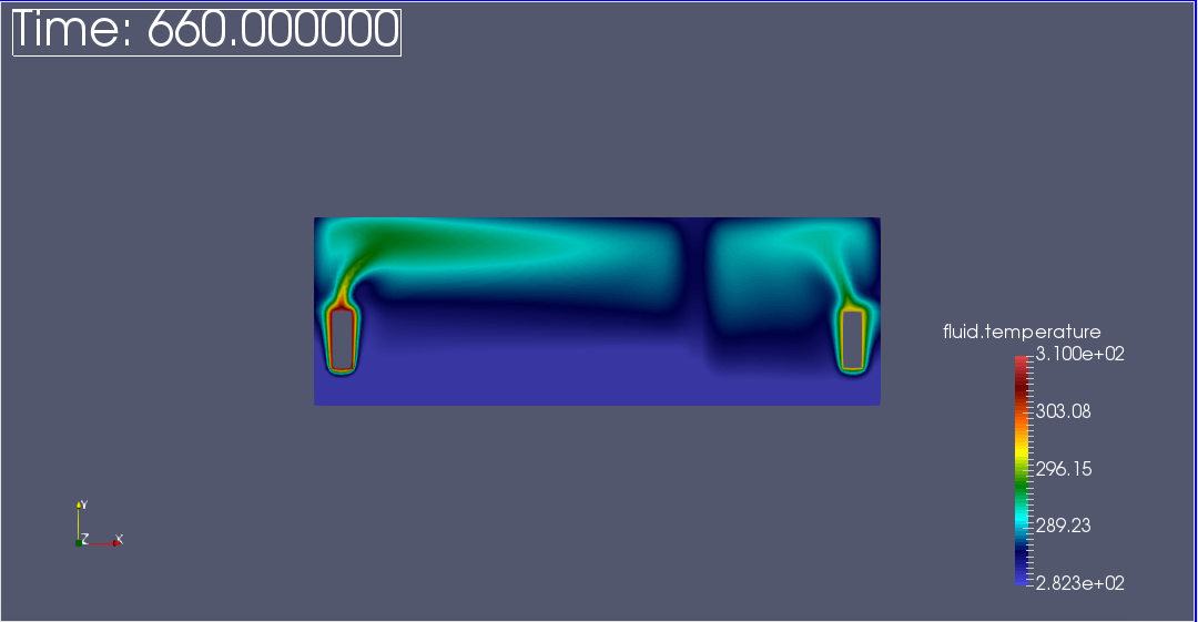
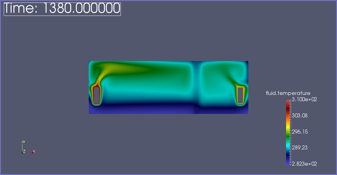
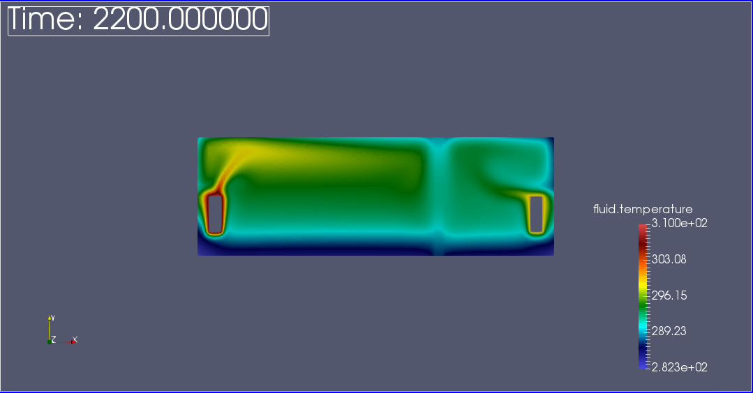
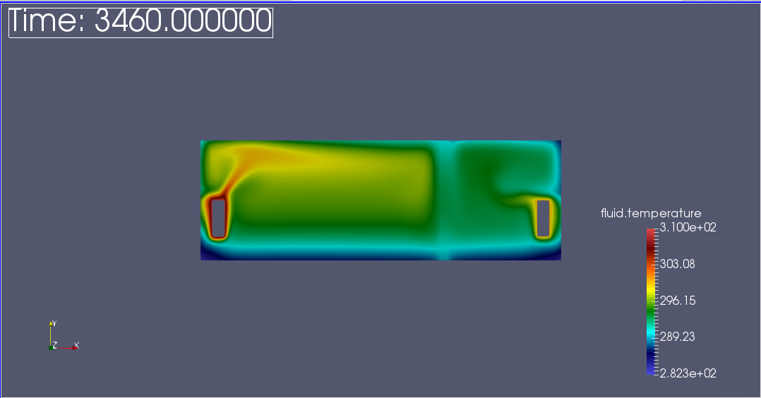
We observe that the flow circulate from the bottom to the top. The cooler fluid in bottom is heated, then becomes less dense and rises. The process continues, forming a convection concurrent and tranfers heat energy around the domain.
|
|
|
|
|
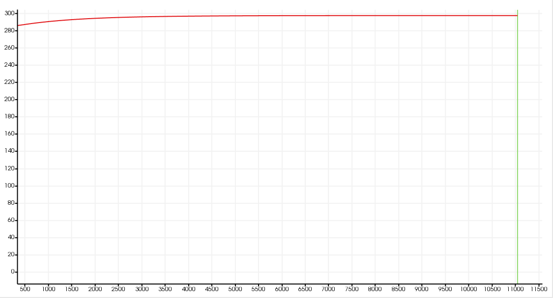
The graph show the steady state of temperature at 300K in all domains.
|
|