 .pdf
.pdf
Solenoïd Benchmark
An analytical solution of the elasticity equation exists in an infinitely long solenoid. Such a geometry has the advantage to be axisymetrical, we can first expresse the solution with cylindrical coordinates.
1. Running the case
The command line to run this case is
mpirun -np 4 feelpp_toolbox_solid --case "github:{path:toolboxes/solid/Solenoid}"2. Definition
2.1. Equilibrium equation in cylindrical coordinates
The analytical solution comes from the electromagnetism equations, indeed this case of a soleinoid crossed by an electric current can model the behaviour of a resistive magnet. The volumic forces \(\mathbf{f}\) of the equilibrium equation are consequently dependent on the current density \(\mathbf{J}\) and the induced magnetic field \(\mathbf{B}\), which gives :
We will use the following notations:
We consider here that the current distribution in the soleinoid is uniform. That means that \(J_{\theta}\) is constant, and \(J_r = J_z = 0\). The volumic forces \(\mathbf{J} \times \mathbf{B}\) becomes :
The revwriting of the equilibrium equation in cylindrical coordinates gives :
The axisymetrical properties of this geometries means that the displacement is invariant with respect to \(\theta\).
Furthermore, the soleinoid we consider has the particularity to be infinitely long, so there is no displacement along \(z\) axis.
We can consequently get rid of all derivatives \(\frac{\partial \cdot}{\partial \theta}\) and \(\frac{\partial \cdot}{\partial z}\).
Finally, we shall note that components \(\sigma_{\theta r}\) and \(\sigma_{zr}\) of the stress tensor \(\bar{\bar{\sigma}}\) are expressed from Hooke’s law only from the components \(v\) and \(w\) of the displacement vector \(\mathbf{u}\), which nullify the two last equations.
Thus, the equilibrium equation is reduced to:
We need to express this equation in terms of the displacement \(\mathbf{u}\), This can be done using Hooke’s law which links the stress tensor to the tensor of small deformation by:
where \(\mu\) and \(\lambda\) are the Lamé coefficients, and the tensor of small deformation is given in cylindrical coordinates by:
Then, using the last two definitions and the properties of the solenoid (axisymmetric and infinitely long), we can rewrite the equilibrium equation as:
2.2. Analytical solution
We want to find an analytical solution of the form :
where \(C_1\) and \(C_2\) are constants, and \(u_p(r)\) a particular solution of the equilibrium equation in cylindrical coordinates.
From Ampére’s theorem and considering that the soleinoid is axisymetrical and infinitely long, we deduce that \(B_r = 0\), and \(B_z\) depends only on \(r\), such that :
with \(r_1\) the internal radius of the soleinoid.
For a uniform distribution of current in the solenoid (\(j_{\theta}\) constant), we deduce that \(B_z\) can be expressed as :
Replacing \(b_z\) with his expression in the equilibrium equation, this gives :
where \(r_2\) is the external radius, \(\alpha = \frac{r_2}{r_1}\) and \(\Delta b_z = B_z(r_1) - B_z(r_2)\).
A particular solution \(u_p(r)\) for this equation is given by:
The constants \(C_1\) and \(C_2\) are set by the boundary conditions, we consider here that there is no surface forces. That gives \(\bar{\bar{\sigma}}\cdot\mathbf{n} = 0\) on internal and external radius, that is \(\sigma_{rr}(r_1)=\sigma_{rr}(r_2)=0\).
Using the definition of \(u_{cyl}\) in
we can solve the system to find the constants:
The final step is to translate this analytical solution \(u_{cyl}(r)\) into cartesian coordinates to obtain the analytical cartesian displacement \(\mathbf{u}_{cart}\):
2.3. Geometry
We use a solenoïd of thickness one with \(r_1=1\) and \(r_2=2\) and with a length sufficiently important (\(l=10\,r_2\)) so that the influence of the top and of the bottom of the geometry, which are supposed not to exist, is close to zero.
2.4. Boundary conditions
The boundary conditions taken into account for the analytical solution have to be reproduced for the simulation. That means null pressure forces on internal and external radius, and displacement set to zero (Dirichlet) on the top and on the bottom to keep only the radial component.
We set:
-
\(\mathbf{u} = 0\) on \(\Gamma_{top}\cup\Gamma_{bottom}\)
-
\(\bar{\bar{\sigma}}\cdot \mathbf{n} = 0\) on \(\Gamma_{int}\cup\Gamma_{ext}\)
-
\(\mathbf{f} = \begin{pmatrix} \frac{x}{\sqrt{x^2+y^2}}5000(10+20(\sqrt{x^2+y^2}-1))\\ \frac{y}{\sqrt{x^2+y^2}}5000(10+20(\sqrt{x^2+y^2}-1))\\ 0 \end{pmatrix}\) in \(\Omega\)
3. Inputs
We use the following parameters:
| Name | Value |
|---|---|
\(E\) |
\(2.1e^6\) |
\(\nu\) |
\(0.33\) |
\(\mathbf{f}\) |
\(\begin{pmatrix} \frac{x}{\sqrt{x^2+y^2}}5000(10+20(\sqrt{x^2+y^2}-1))\\ \frac{y}{\sqrt{x^2+y^2}}5000(10+20(\sqrt{x^2+y^2}-1))\\ 0 \end{pmatrix}\) |
4. Output
We compare the radial component of the displacement on the segment \(z=l/2\), \(y=0\) and \(x\in \lbrack 1,2\rbrack \).
5. Results
Here are the analytical and the computed \(x\) component of the displacement. This has been obtain with a characteristic size of \(0.1\) and \(646 233\) dofs.
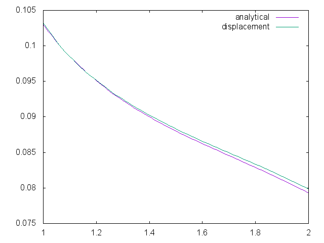
We can see that the errors grows as we approach the external radius. But the max of the error is \(5e^{-4}\) and it converges as the characteristic size decreases.