.pdf
.pdf
Boundary Layer Development Benchmark
Analysis Type: Convective heat transfer
| this benchmark has been published by NAFEMS, it is being implemented/tested using Feel++ |
Introduction
The boundary layer is the area of the viscous flow near the wall where the fluid velocity changes from the wall velocity (which is zero for a stationary wall to the free stream velocity ( \(u_{\infty}\) ). This means that friction forces that oppose the free stream motion of the fluid are confined to this relatively thin layer. As such, the boundary layer is characterized by large flow gradients.
The development of a convective boundary layer over a flat plate is a mathematically well-defined problem for which an analytical approximation exists. The present case describes the development of the momentum as well as the thermal boundary layer over an isothermal plate. The solution of the problem allows calculation of the wall friction and the heat transfer between the wall and the fluid flow.
1. Objectives
The laminar flow case examines the extent of numerical diffusion associated with discretisation of the convection terms in the momentum and energy equations. The introduced numerical error is manifested by the accelerated growth of the momentum and thermal boundary layers, which increases the boundary layer thickness and reduces velocity and temperature gradients.
Deficiencies in the convection term discretization may also be exposed in the form of convergence problems due to unbounded amplification of local disturbances.
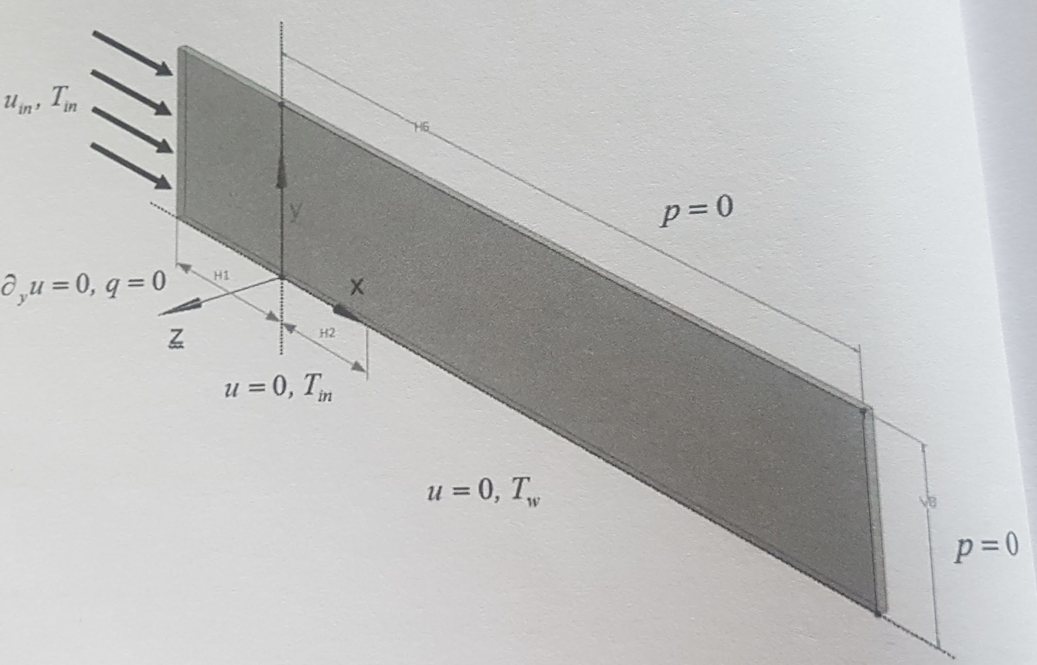
2. Geometry
-
Length of the upstream section \((\mathrm{H} 1)\) is \(2.0 \mathrm{m}\)
-
Length of the unheated section \((\mathrm{H} 2)\) is \(1.0 \mathrm{m}\)
-
Length of the momentum boundary layer development (H6) is \(10.0 \mathrm{m}\)
-
Domain height (V8) is 2.0 \(\mathrm{m}\)
-
Domain width is \(0.1 \mathrm{m}\) (although not important due to the case twodimensionality).
3. Case Definition
-
The inflow with uniform velocity \(u_{i n}=1.0 \mathrm{m} / \mathrm{s}\) and temperature \(T_{i n}=20^{\circ} \mathrm{C}\) is set for the inlet.
-
The momentum boundary layer develops due to the imposed no-slip wall boundary conditions along the bottom wall.
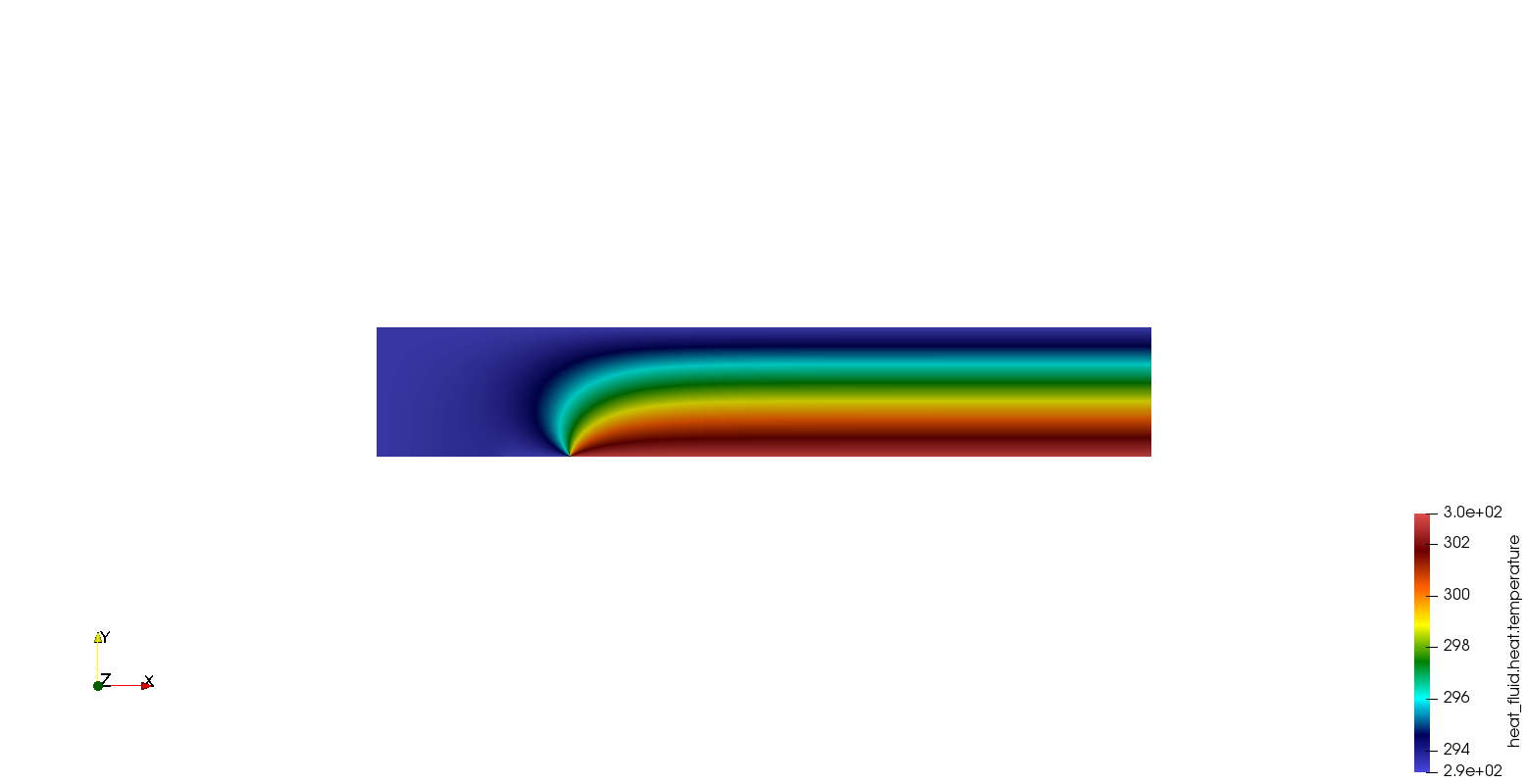
*Similarly, formation of the thermal boundary layer is initiated by a sudden increase in the wall temperature from \(T_{i n}=20^{\circ} \mathrm{C}\) to \(T_{w}=\) \(30^{\circ} \mathrm{C}\)
4. Fluid Properties
The following fluid material properties shall be used:
-
\(\cdot \rho\) is density of \(1.0 \mathrm{kg} / \mathrm{m} 3\)
-
\(\mu\) is dynamic viscosity of \(0.0012 Pa s\);
-
\(c_{p}\) is specific heat capacity of \(1000.0 \mathrm{J} / \mathrm{kgK}\)
-
\(\therefore \lambda\) is thermal conductivity of \(0.5 \mathrm{W} / \mathrm{mK}\)
The fluid material properties are adjusted to yield an accelerated growth of the momentum and the thermal boundary layer in order to avoid the need for a very long simulation domain in the x-direction.
6. Boundary Conditions
-
Uniform velocity and temperature at the inlet: \(u_{i n}=1.0 \mathrm{m} / \mathrm{s}\) and \(T_{i n}=20^{\circ} \mathrm{C}\)
-
Initial section of the bottom wall (H1) with the adiabatic free-slip wall boundary conditions: \(\partial_{y} u=0.0 \mathrm{s}^{-1}\) and \(q=0.0 \mathrm{W} / \mathrm{m}^{2}\)
-
Unheated section of the bottom wall (H2) with the no-slip boundary condition and the temperature: \(u=0.0 \mathrm{m} / \mathrm{s}\) and \(T_{i n}=20^{\circ} \mathrm{C}\)
-
The no-slip boundary condition \(u=0.0 \mathrm{m} / \mathrm{s},\) and the elevated temperature \(T_{w}=30^{\circ} \mathrm{C}\) assigned to the rest of the bottom wall (H6-\(\mathrm{H} 2)\)
-
For the top and the outlet boundaries, a zero relative pressure is appropriate;
-
For the vertical \(X-Y\) surfaces, symmetry or equivalent conditions shall be used.
7. Output
The exact and closed-form solution for the velocity \((u)\) and the temperature \((T)\) distribution across the boundary layer does not exist.
A simplified set of fluid flow transport equations yields the Blasius solution of the boundary layer problem [1]: \(u=\frac{u_{i n}}{2}\left(\eta f^{\prime}-f\right) R e_{x}^{-1 / 2},\) where \(\eta=y \sqrt{\frac{\rho u_{i n}}{\mu x}}, \quad R e_{x}=\frac{\rho u_{i n} x}{\mu}\) for which \(f\) is obtained numerically or tabulated. For that reason, compare:
-
momentum boundary layer thickness \(\delta_{99},\) where \(u=0.99 u_{\max },\) at intervals along the domain with the expression derived from the Blasius solution [2] \(\delta_{99} \sim 5.0 \times R e_{x}^{-1 / 2}\) for \(x \geq 0\)
-
local wall friction coefficient \(C_{f}=2 \mu \partial_{y} u / \rho u_{i n}^{2}\) with the expression derived from the Blasius solution [2] \(C_{f}=0.664 R e_{x}^{-1 / 2}\) for \(x \geq 0\)
-
local Nusselt number \(N u=\partial_{y} T x /\left(T_{w}-T_{i n}\right)\) with the expression derived from the Pohlhausen’s solution [3] \(N u=0.332 R e_{x}^{1 / 2} \operatorname{Pr}^{1 / 3}\left(1-\left(\frac{x_{\text {ini}}}{x}\right)^{3 / 4}\right)^{-1 / 3}\) for \(x \geq x_{\text {ini}}\) where:
-
\(P r=c_{p} \mu / \lambda\) Prandtl number
-
\(x\) distance from the leading edge
-
\(x_{i n i}\) initial unheated distance (H2)
-
Diagrams of \(\delta_{99}, C_{f}\) and \(N u\) as a function of the distance from the trailing edge ( \(x\) ) shall be prepared. They should include the results obtained with the CFD simulations and the analytical approximations.
The quadratic mean (or RMS) of the deviation can be used to quantify the level of agreement between both sets of results.
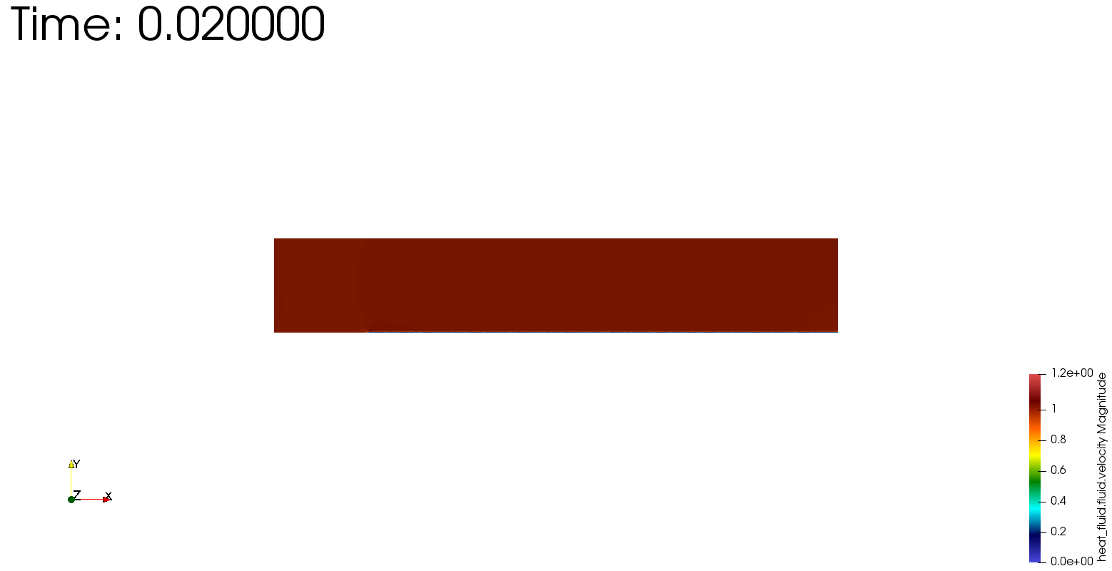
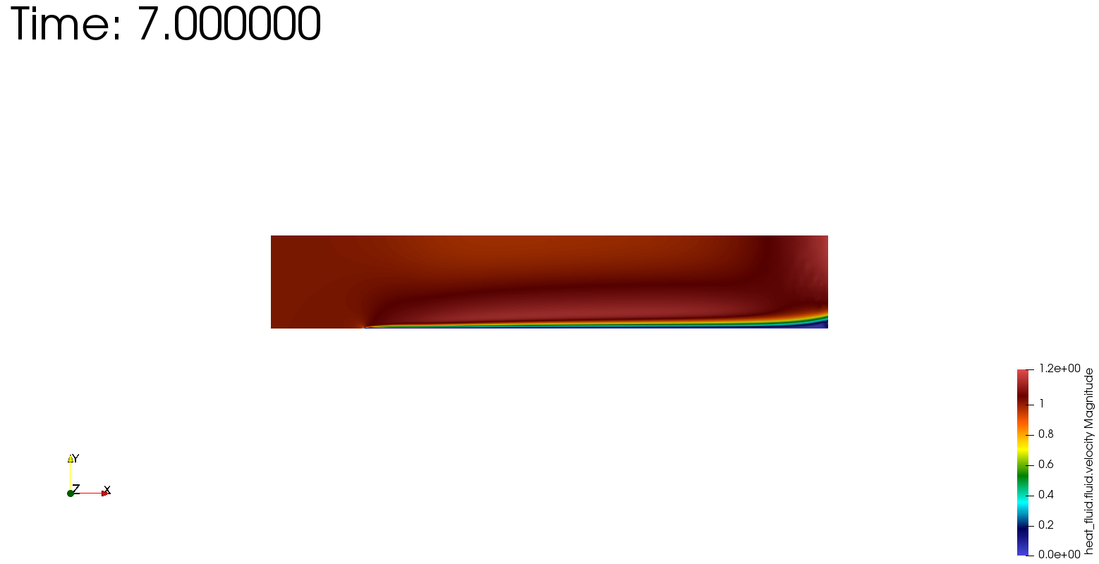
8. Simulation
The geometry file is available on Github here.
To visualize the momentum boundary layer thickness \(\delta_{99}\), we defin in the geometry vertical lines every meter :
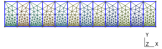
As the main phenomenon stands on the bottom of the area, we need to have a thinier mesh here.
| In the repository, you can find a geo file in 3D of the geomerty, but it isn’t configured with the case yet. |
9. Results
|
|