 .pdf
.pdf
Inflatable structure
We will provide a 2D example of fluid-structure interaction taken from the article
-
Küttler, U., Förster, C. & Wall, W.A. Comput Mech (2006) 38: 417. doi.org/10.1007/s00466-006-0066-5
with different solid and fluid parameters, that were inspired by Jimmy Mullaert PhD thesis
-
Jimmy Mullaert. Numerical methods for incompressible fluid-structure interaction. General Mathematics [math.GM]. Université Pierre et Marie Curie - Paris VI, 2014.
1. Introduction
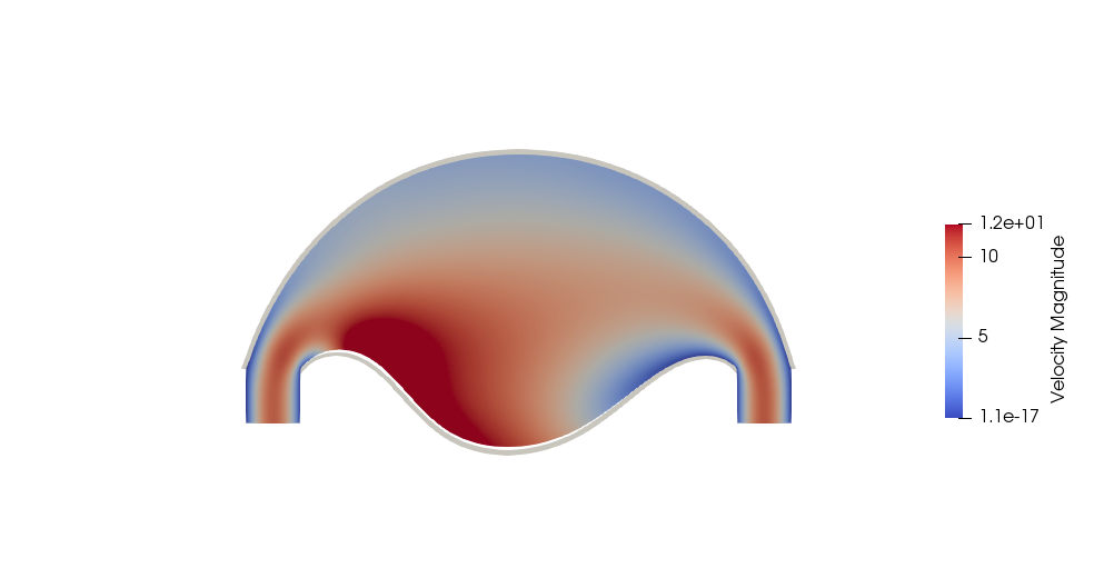
We will simulate the inflation of a deformable semicircular structure under continuous immission of an incompressible fluid. The structure is made of two solid layers, the above one being more elastic than the bottom one. We will see that, while the top structure deformates significantly, the bottom one will be essentially undeformed until it collapses, due to the high pressure between the two.
In this model, fluid’s boundary conditions are only of Dirichlet type. It is known that this situation is difficult to be tackled using partitioned solvers with Dirichlet-Neumann discretization of FSI coupling conditions. There are two reasons for this: the so called incompressiblity condition dilemma, and the fact that pressure’s absolute value is not known. The incompressibility condition dilemma can be described as follows: whenever the structure’s displacement is calculated, it should take into account the fluid’s volume change in the next time step to be admissible and produce an admissible interface velocity (compatible with incompressibility condition inside the fluid subdomain). In a Dirichlet-Neumann approach, this is not the case: in fact, the new interface, computed with Neumann conditions on the solid subproblem, and the new interface velocity computed through finite differences do not, a priori, satisfy such constraint. The pressure issue, finally, can be solved by prescribing a pressure value on the boundary of the fluid domain. We will perform the simulation applying a Generalized Robin-Neumann coupling condition to avoid these problems.
2. Model/Geometry
The numerical domain is shown in the figure below. We will indicate by \(\Omega_f^*\) and \(\Omega_s^*\) the initial fluid and solid subdomain, respectively. \(\Omega_s^*\) is the ensemble of the two thin structures in the following figure.
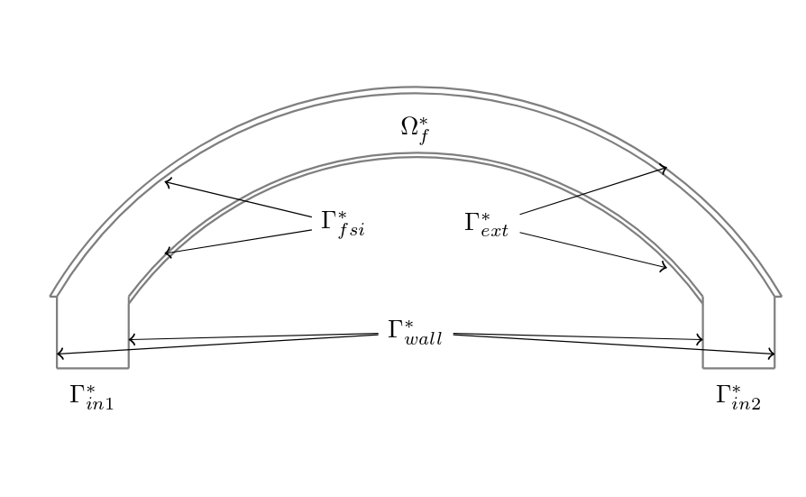
The distance between the two pillars, each of height and extension \(1 m\), is \(8 m\). The curved elements are arcs of circumference: they are \(0.1 m\) thick in the middle of the span and \(1 m\) apart from each other. The inferior side of the bottom structure is \(2.9 m\) above the ground at its peak. The two structures are fixed on their respective extremities, each measuring \(0.1 m\).
3. Materials and Boundary Conditions
We employ materials having the following properties:
| Name | Description | Nominal Value | Units |
|---|---|---|---|
\(E\) |
Young modulus |
\(9 \cdot 10^5\) |
\(kg/m^2\) |
\(\nu\) |
Poisson coefficient |
\(0.3\) |
|
\(\rho_s\) |
Density |
\(500\) |
\(kg/m^3\) |
| Name | Description | Nominal Value | Units |
|---|---|---|---|
\(E\) |
Young modulus |
\(9 \cdot 10^7\) |
\(kg/m^2\) |
\(\nu\) |
Poisson coefficient |
\(0.3\) |
|
\(\rho_s\) |
Density |
\(500\) |
\(kg/m^3\) |
| Name | Description | Nominal Value | Units |
|---|---|---|---|
\( \mu_f \) |
Dynamic viscosity |
\(9.0\) |
\(kg/(ms)\) |
\(\rho_f\) |
Density |
\(1.0\) |
\(kg/m^3\) |
Solids are modeled using a Neo-Hookean hyperelastic model and the fluid by a Newtonian model.
We impose the following boundary conditions on the domain:
-
on \(\Gamma_{1}^*\) and \(\Gamma_2^*\), an inflow parabolic Dirichlet condition on fluid velocity, with slightly different maximal values to avoid perfect symmetry in the structure (\(10\) and \(10.2\) \(m/s\));
-
on \(\Gamma_{wall}^*\), a homogeneous Dirichlet condition on fluid velocity : \(\boldsymbol{u}_f = \boldsymbol{0}\);
-
on \(\Gamma_{ext}^*\), a homogeneous Neumann condition on solid forces \(\boldsymbol{\sigma}_s = \boldsymbol{0}\);
-
on \(\Gamma_{fixed}^*\), a zero displacement condition on the solid side \(\boldsymbol{\eta}_s = \boldsymbol{0}\) and a homogeneous Dirichlet condition on the fluid side;
-
on \(\Gamma_{fsi}^*\) :
where \(\boldsymbol{n}_f\) is the outer unit normal vector from \(\partial \Omega_f^*\).
We will suppose that the fluid experiences a constant volume force of value \(\boldsymbol{f} = (0,-1)\) directed in the negative \(y\) direction.
The inflow parabolic profile is imposed progressively: up to time \(t=1\) it is multiplied by \(\sin(\frac{\pi t}{2})\).
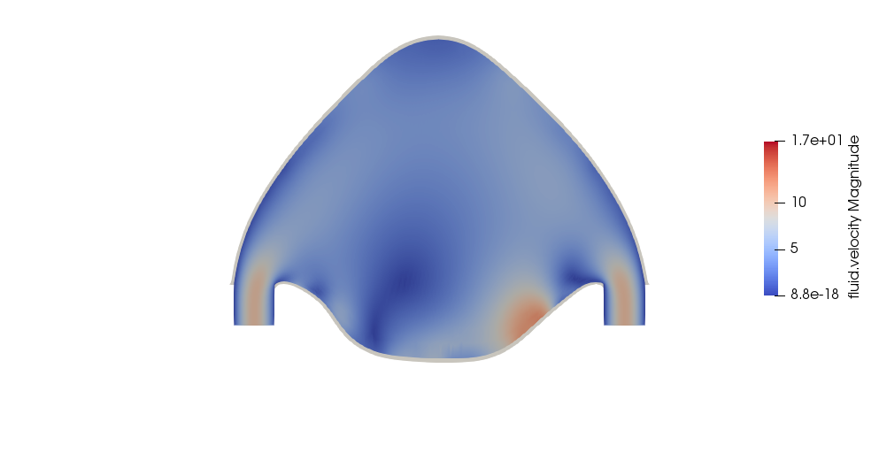
4. Results
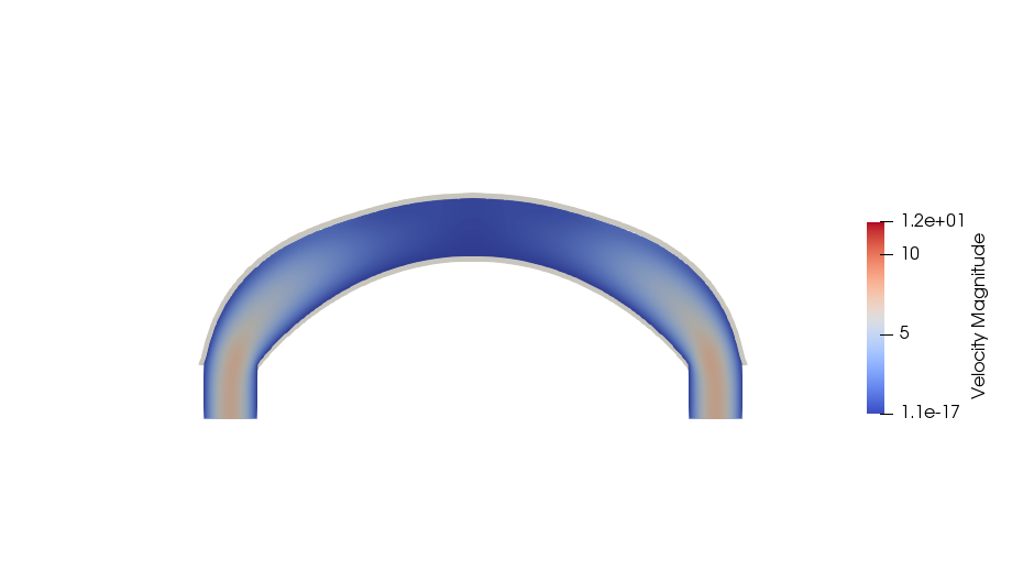
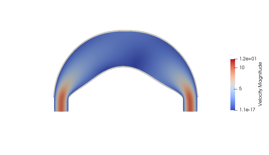
We collect some results that we have obtained from the simulations. In particular we show the velocity modulus at different time-steps
5. Methodology
These results were obtained by using the Feel++ 2D Fluid Structure Interaction application. The simulation was run on 24 processors using the following command:
$ mpirun -np 24 /usr/local/bin/feelpp_toolbox_fsi_2d --config-file structure-balloon.cfgThe information regarding material properties and boundary conditions were specified in .json files, the geometry in the .geo file and the numerical specifications characterizing the simulation (solvers, preconditioners, constitutive models, …) in the .cfg file. The material parameters are specified as follows:
    "Materials":
    {
        "Fluid": {
            "rho":"1",
            "mu":"9"
        }
    },
"Materials":
{
"Top-solid": {
"E":"9e5",
"nu":"0.3",
"rho":"5e2"
},
"Bottom-solid": {
"E":"9e7",
"nu":"0.3",
"rho":"5e2"
}
},The boundary conditions, instead, are specified in the following manner:
    "BoundaryConditions":
    {
        "velocity":
        {
            "Dirichlet":
            {
		"wall":
		{
		    "expr":"{0,0}"
		},
		"solid-fixed":
		{
		    "expr":"{0,0}"
		}
            },
            "interface_fsi":
            {
                "fsi":
                {
                    "expr":"0"
                }
            }
	},
	"fluid":
	{
	    "inlet":
	    {
		"inlet1":
		{
		    "shape":"parabolic",
		    "constraint":"velocity_max",
		    "expr":"10*(sin(pi*t/2)*(t<1)+(1-(t<1))):t"
		},
		"inlet2":
		{
		    "shape":"parabolic",
		    "constraint":"velocity_max",
		    "expr":"10.2*(sin(pi*t/2)*(t<1)+(1-(t<1))):t"
		}
	    }
	},
	"VolumicForces":
	{
	    "":
	    {
		"expr":"{0,-1}"
	    }
	}
    },
"BoundaryConditions":
{
"displacement":
{
"Dirichlet":
{
"solid-fixed":
{
"expr":"{0,0}"
}
},
"interface_fsi":
{
"fsi":
{
"expr":"0"
}
},
"Neumann_scalar":
{
"free-solid":
{
"expr":"0"
}
}
}
},