.pdf
.pdf
Example Toolboxes 2D building
\(\quad\)In this example, we will build a thermal model of the building. The strategy is to complicate the simple 2D model by adding physical parameters and using equivalent approximation terms and numerical methods of finite element. The Toolboxe heat will be used to solve the problem.
\(\quad\)The construction of the model requires a well-posed problem, that is to say, if from a theoretical point of view the equations have many unique solutions. For this, we need to make the weak formulations of the equations we will use. This is a part that remains important, because if the problem is poorly posed, then we may have no solution or several. This gives false numerical schemes and the simulations made may be wrong.
1. Running the case
The command line to run this case is
mpirun -np 8 feelpp_toolbox_heat --case "github:{repo:toolbox,path:examples/modules/heat/examples/2Dbuilding}"2. Data files
The case data files are available in Github here
3. 2D thermal model
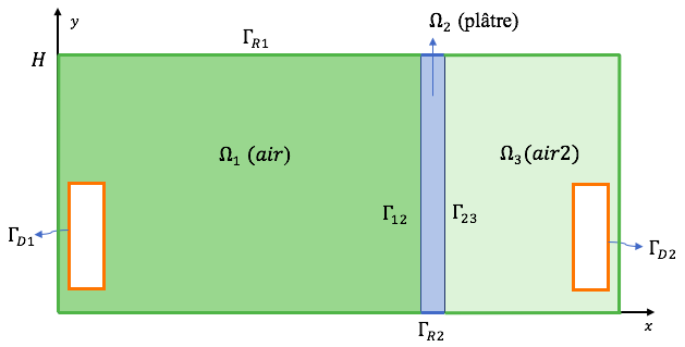
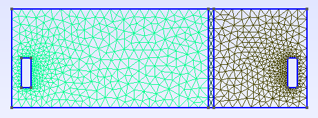
\(\quad\)The 2D thermal model of two parts separated by plaster is considered. It is an object of \(\mathbb {R} ^ 2\), it is subdivided into different domains \(\Omega_i, i = 1,2,3\) (see the image). The sources of heat \(heater_i, i = 1,2\) are the two radiators each of which is located downstairs in each room. The heat \(T\) released in the subdomains is calculated thanks to the equation of heat transfer.
We use model multi-physique of heat tranfert with \(k_i (y)\) which is the thermal conductivity which depends the coordinate from the stem height:[y], and we have \(0 \leq y \leq H\).
\(\ quad\) We notice that in this first model, taking the parameter \(k_i (y)\) increasing linear, varied according to the height, we can simulate the effect that the cold air is at the bottom and the warm air diffuses towards the ceiling. This is the effect of natural convection. This is an improvement of the model with \(k\) constant.
|
The conditions at the edges:
-
Condition of Dirichlet
-
Condition of Robin
Conditions at the interface \(\Gamma_{ij} = \Omega_i \cap \Omega_j\)
Initial condition to \(t = 0s\)
3.1. Input
| Notation | Description | Value | Unit | Note |
|---|---|---|---|---|
Paramètres globale |
||||
\(t\) |
times |
s |
||
\(T\) |
temperature |
\(K\) |
||
\(T_{ext}\) |
outside temperature |
280 |
\(K\) |
|
\(T_0\) |
initial temperature |
280 |
\(K\) |
|
\(H\) |
height |
\(1,2,3\) |
\(m\) |
|
Air |
||||
\(k_1(y)\) |
thermal conductivity |
\(W.m^{-3}.K^{-1}\) |
||
\(k_1^{ground}\) |
k_1(0) |
\(1.,1.5.,2.\) |
\(W.m^{-3}.K^{-1}\) |
|
\(k_1^{roof}\) |
k_1(H) |
\(4.,5.,6.\) |
\(W.m^{-3}.K^{-1}\) |
|
\(\rho_1\) |
mass volumique |
1 |
\( kg/(m^3) \) |
|
\(C_1\) |
thermal capacity |
1004 |
\( J/(kg*K) \) |
|
\(h_1\) |
heat transfer coefficient |
1.0/(0.06+0.01/0.5 + 0.3/0.8 + 0.20/0.032 +0.016/0.313 +0.14) |
\( W.m^{−2}.K^{−1} \) |
|
\(heater_1\) |
heat source |
310 |
\(K\) |
|
Air2 |
||||
\(k_2(y)\) |
thermal conductivity |
\(W.m^{-3}.K^{-1}\) |
||
\(k_2^{ground}\) |
k_2(0) |
\(1.,1.5.,2.\) |
\(W.m^{-3}.K^{-1}\) |
|
\(k_2^{roof}\) |
k_2(H) |
\(4.,5.,6.\) |
\(W.m^{-3}.K^{-1}\) |
|
\(\rho_2\) |
mass volumique |
1 |
\( kg/(m^3) \) |
|
\(C_2\) |
thermal capacity |
1004 |
\( J/(kg*K) \) |
|
\(h_2\) |
heat transfer coefficient |
1.0/(0.06+0.01/0.5 + 0.3/0.8 + 0.20/0.032 +0.016/0.313 +0.14) |
\( W.m^{−2}.K^{−1} \) |
|
\(heater_2\) |
heat source |
300 |
\(K\) |
|
Plâtre |
||||
\(k_3(y)\) |
thermal conductivity |
\(W.m^{-3}.K^{-1}\) |
||
\(k_3^{ground}\) |
k_3(0) |
\(0.25\) |
\(W.m^{-3}.K^{-1}\) |
|
\(k_3^{roof}\) |
k_3(H) |
\(0.25\) |
\(W.m^{-3}.K^{-1}\) |
|
\(\rho_3\) |
mass volumique |
150 |
\( kg/(m^3) \) |
|
\(C_3\) |
thermal capacity |
1000 |
\( J/(kg*K) \) |
|
\(h_3\) |
heat transfer coefficient |
1.0/(0.06+0.01/0.5 + 0.3/0.8 + 0.20/0.032 +0.016/0.313 +0.14) |
\( W.m^{−2}.K^{−1} \) |
|
4. Implementation
Note on the definition of the function \(k_i(y)\) in the .cfg file
directory=applications/ibat/heat-transfert/toolbox
case.dimension=2
mesh.filename=$cfgdir/thermo2d.geo gmsh.hsize=0.01#0.05
filename=$cfgdir/thermo2d.json
initial-solution.temperature=280
#do_export_all=true #verbose=1 #verbose_solvertimer=1 reuse-prec=1 pc-type=gamg
order=2
time-step=300 time-final=5e4 restart.at-last-save=true
{
    "Name": "Thermo dynamics",
    "ShortName":"ThermoDyn",
    //"Model":"Thermic",
    "Parameters":
    {
         "kground":"0.001",
         "kroof":"2.9"
    },
    "Materials":
    {
        "air":
        {
	    "markers":"air",
            //"k":"2.9",//[0.0262 W/(m*K) ]
            "rho":"1",
            "mu":"2.65e-2",
            "k":"kground+ (y^6)*(kroof-kground):y:kroof:kground",
            "Cp":"1004"
        },
        "air2":
        {
	    "markers":"air2",
            //"k":"2.9",//0.0262[ W/(m*K) ]
            "rho":"1",
            "mu":"2.65e-2",
            "k":"kground+ (y^6)*(kroof-kground):y:kroof:kground",
            "Cp":"1004"
        },
        "internal-walls":
        {
	    "markers":"internal-walls",
            "k":"0.25",//[ W/(m*K) ]
            //"k11":"0.0262"//[ W/(m*K) ]
            "Cp":"1000", //[ J/(kg*K) ]
            "rho":"150" //[ kg/(m^3) ]
        }
    },
    "BoundaryConditions":
    {
        "temperature":
        {
            "Dirichlet":
            {
                "heater1": { "expr":"310"/*"330"*/ },
                "heater2": { "expr":"310"/*"320"*/ }
            },
            "Robin":
            {
                "exterior-walls":
                {
                    "expr1":"1.0/(0.06+0.01/0.5 + 0.3/0.8 + 0.20/0.032 +0.016/0.313 +0.14)",// h coeff
		    "expr2":"280"// temperature exterior
                },
		"exterior-walls-iw":
		{
		    "expr1":"1.0/(0.06+0.01/0.5 + 0.3/0.8 + 0.20/0.032 +0.016/0.313 +0.14)",// h coeff
		    "expr2":"280"// temperature exterior
		}
            }
        }
    },
    "PostProcess":
    {
	"Exports":
	{
        "fields":["temperature","pid"]
	}
    }
}
mpirun -np 16 feelpp_toolbox_heat_2d --config-file thermo2d.cfgcase with link to folder which represents a remote data in a github repository.mpirun -np 8 feelpp_toolbox_heat --case "github:{repo:toolbox,path:examples/modules/heat/examples/2Dbuilding}"You can also use some options to change the variables like time-final, taille du maillage hsize, …
mpirun -np 8 feelpp_toolbox_heat --case "github:{repo:toolbox,path:examples/modules/heat/examples/2Dbuilding}" --ts.time-final 30005. Result
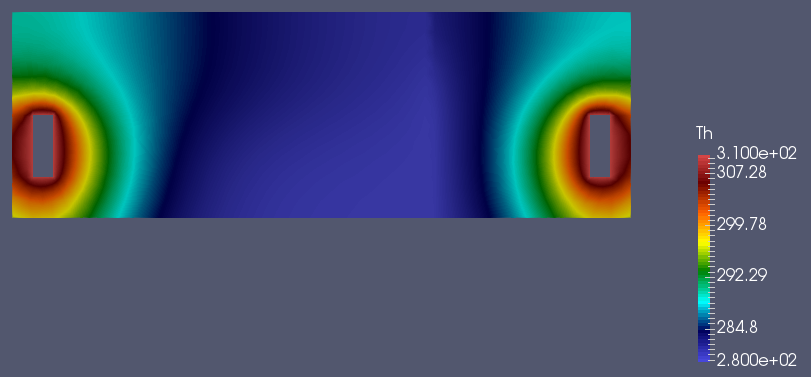
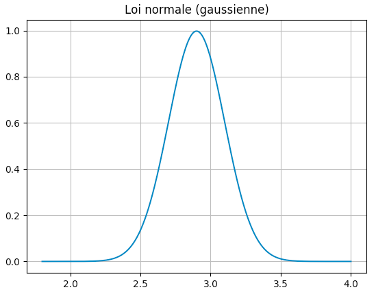
Choose k following an equivalent value \(k_{eq} = 2.9\) (see [1]) then generate the value of \(k^{ground}\) and \(k^{roof}\) follow a normal distribution
|
|
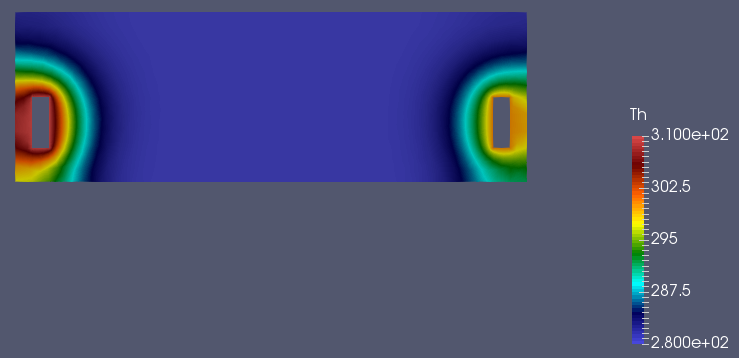
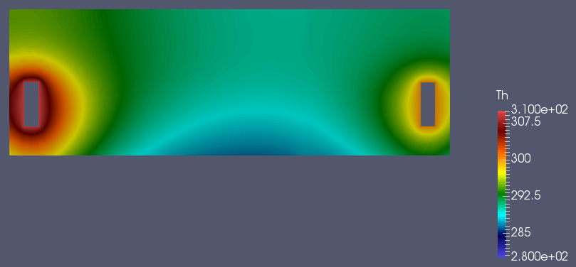
Utilise la fonction \(k(y)\) non linéaire
\(k^{ground} = 0. , k^{roof} = 2.9 , tmax=1000, dt = 0.01\) |
\(k^{ground} = 0. , k^{roof} = 2.9 , tmax=150000, dt = 500\) |
|
|
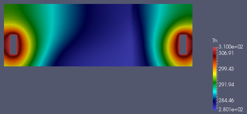
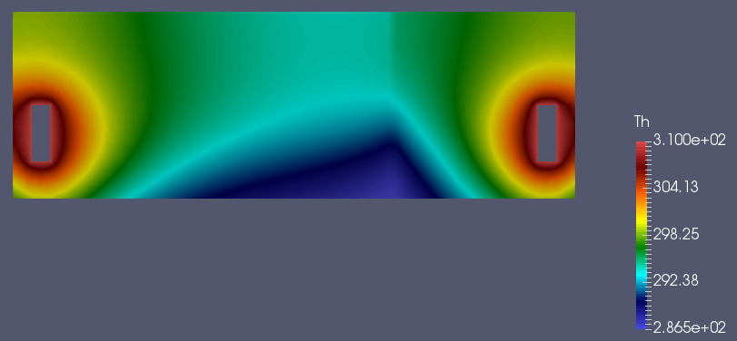
Uses the function \(k(y)\) nonlinear with powerful 6
\(k^{ground} = 0. , k^{roof} = 2.9 , tmax=1000\) |
\(k^{ground} = 0. , k^{roof} = 2.9 , tmax=1000, dt=300\) |
|
|