 .pdf
.pdf
Cyclone
2. Running the case
The command line to run this case is
mpirun -np 4 feelpp_toolbox_fluid --case "github:{repo:toolbox,path:examples/modules/cfd/examples/cyclone}3. Data files
The case data files are available in the GitHub repository:
4. Geometry
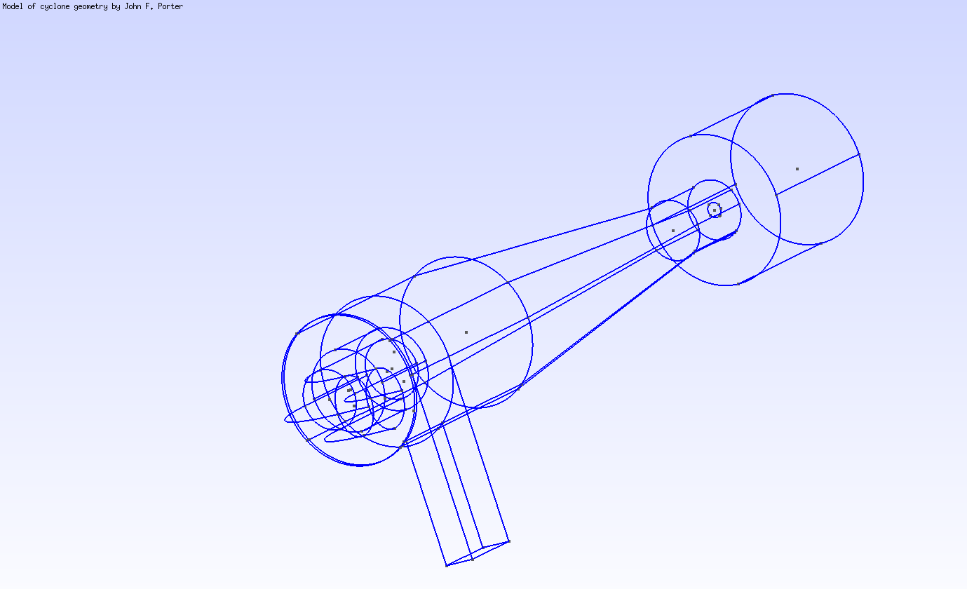
The geometry describes a cyclonic separation device (hydrocyclone) and can be found on Girder
5. Input parameters
| Name | Description | Value | Unit | |
|---|---|---|---|---|
\(\mu_f\) |
fluid velocity |
\(1 \times 10^{-3}\) |
\(Pa.s\) |
|
\(\rho\) |
fluid density |
\(998\) |
\(kg/m^3\) |
6. Model & Toolbox
The model used is a Stokes model. It is described in the CFD toolbox, see Computational Fluid Dynamics
6.1. Materials
"Materials":
{
  "internal_volume":
  {
    "name":"Water",
    "rho":998, // [kg/m^3]
    "mu":1e-3 // [Pa.s]
  }
},
6.2. Boundary conditions
The domain boundary is divided in three parts: the inlet, the outlet and the wall. The wall is the part of the fluid domain boundary which corresponds to the device structure, which is a solid.
6.2.1. Wall
We apply a Dirichlet boundary condition on the wall where the fluid velocity vanishes. The fluid particles at the (fluid) wall are also stuck on the (solid) wall. This means the velocity of the fluid equals the velocity of the solid at the fluid-solid interface. We are only simulating the fluid flow, so the device is considered a non-moving rigid body. Hence, its velocity at all point is zero, and so is the fluid velocity on the wall.
6.2.2. Inlet
We also use a Dirichlet condition for the inlet: we impose the flow rate and a Poiseuille flow (parabolic shaped velocity profile).
6.2.3. Outlet
The outlet is left with a free outflow boundary condition, which means no imposed stress along the normal to the boundary.
"BoundaryConditions":
{
  "velocity":
  {
    "Dirichlet":
    {
      "wall":
      {
        "expr":"{0,0,0}"
      }
    }
  },
  "fluid":
  {
    "inlet":
    {
      "inlet":
      {
        "expr":"1e-3", // [m^3/s]
        "shape":"parabolic", // constant, parabolic
        "constraint":"flow_rate" // velocity_max, flow_rate
      }
    },
    "outlet":
    {
      "gas_outlet":
      {
        "expr":"0"
      }
    }
  }
},
7. Outputs
The fields of interest for this example are the velocity, the pressure and the parallel process id (pid). The pid helps to see how the mesh was partitioned for parallel processing. In the 3D view below, when selecting the pid in the first dropdown list, each color corresponds to a subdomain assigned to and processed by a CPU core.
"PostProcess":
{
  "Exports":
  {
    "fields":["velocity","pressure","pid"]
  }
}