Mass transport in a Stokes flow in a pipe

Table of Contents

1. Running the model
2. Data files
- 2.1. Json file
- 2.2. Cfg file
3. Geometry
- 3.1. Model & Toolbox
4. Input parameters
5. Numerical Experiments

1. Running the model

The command line to run this pipestokes case

mpirun -np 4 feelpp_toolbox_fluid --case "github:{repo:toolbox,path:examples/modules/heatfluid/examples/pipestockes_mass}"

2. Data files

2.1. Json file

JSON file - [Edit the file]

2.2. Cfg file

CFG file - [Edit the file]

3. Geometry

3.1. Model & Toolbox

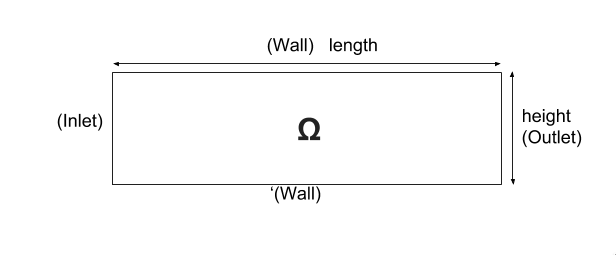
We consider a 2D model representative of a laminar incompressible flow around an obstacle. The flow domain, named \(\Omega_f\), is contained into the rectangle \( \lbrack 0,Long \rbrack \times \lbrack 0,Haut \rbrack \). It is characterised, in particular, by its dynamic viscosity \(\mu_f\) and by its density \(\rho_f\).

The goal of this benchmark is to couple the Stockes equations and the Concentration equations.
we remind that the Stokes equation are

\[ \left\{ \begin{aligned} \boldsymbol{\mu}\boldsymbol{\Delta u}+\boldsymbol{\nabla p}=f\\ \boldsymbol{\nabla}\cdot\boldsymbol{u}=0 \end{aligned} \right.\]

with \(\boldsymbol{\mu}\) is the dynamic viscosity, \(\boldsymbol{p}\) is the pressure ,\(f\) the source and u the velocity.

And the Concentration equations is

\[\begin{array}[c]{rl} \frac{\partial C}{\partial t} + \boldsymbol{u} \cdot \nabla C - \nabla \cdot \left( D_{p} \nabla C \right) = 0, \quad \text{ in } \Omega \end{array}\]

With \(D_{p}\) the diffusion coefficient on the plasma.

We used the heat fluid toolbox, we replaced the temperature by the Concentration, k by \(D_{p}\), and we posed \(\rho C_{p}=1\) to have the same kind of equations.

4. Input parameters

The following table displays the various fixed and variables parameters of this test-case.

Table 1. Fixed and Variable Input Parameters
Name	Description	Units
\(u\)	fluid velocity	\(m/s\)
\(\rho\)	density of the fluid	\(kg/m^3\)
\(\nu\)	dynamic viscosity	\(kg/(m×s)\)
\(p\)	pression	\(Pa\)
\(f\)	source term	\(kg/(m^3×s)\)
\(C_p\)	thermal capacity	\(J/(kg∗K)\)
\(T\)	Temperature	\(K\)
\(Q\)	heat source	\(W.m^{-3}\)
\(D_{p}\)	the diffusion coefficient on the plasma	\(\mu m²/s\)

4.1. initial condition

For the fluid:

We use a parabolic velocity profile, in order to describe the flow inlet by \( \Gamma_{in} \), which can be express by

\[v_{inlet}=D y(height-y)\]

To determine \(D\), we know that for \(y=\frac{height}{2}\) we have the maximal velocity, so

\[D=\frac{v_{max}}{\frac{height}{2}\left(height-\frac{height}{2}\right)}\]

For the Concentration:

We give as source this Concentration

\[ C_{in}=300*(y>0.15)*(y<0.5)+(293.15*(y<(0.15-1e-9)))+(293.15*(y>(0.5-1e-9)))\]

4.2. Materials

   "Materials":
    {
        "Fluid":{
            "rho":"1.0",
            "mu":"1.0",
            "k":"2400.e-6",
            "Cp":"1.0"

        }
    }

4.3. Boundary conditions

For the fluid:

We set

On \(\Gamma_{in}\), an inflow Dirichlet condition : \( \boldsymbol{u}_f=(v_{in},0) \)
On \(\Gamma_{wall}\) and \(\Gamma_{obst}\), a homogeneous Dirichlet condition : \( \boldsymbol{u}_f=\boldsymbol{0} \)
On \(\Gamma_{out}\), a Neumann condition : \( \boldsymbol{\sigma}_f\boldsymbol{ n }_f=\boldsymbol{0} \)

For the Concentration:

On \(\Gamma_{in}\), an inflow Dirichlet condition : \( \boldsymbol{C}_f=C_{in} \)

----
    "BoundaryConditions":
   {
       "velocity":
       {
           "Dirichlet":
           {
               "inlet":
               {
                  "expr":"{D*y*(height-y),0}:y:height:D"
               },
               "wall1":
               {
                   "expr":"{0,0}"
               },
               "wall2":
               {
                   "expr":"{0,0}"
               }
           }
       },
       "fluid":
       {
           "outlet":
           {
               "outlet":
               {
                   "expr":"0"
               }
           }
       },
       "temperature":
       {
           "Dirichlet":
           {
               "inlet":
               {
                   "expr":"300*(y>0.15)*(y<0.5)+(293.15*(y<(0.15-1e-9)))+(293.15*(y>(0.5-1e-9))):y"
               }
           }
       }
   }

4.4. Fields

We are intersting in the visualisation of the three fields : the velocity, the pressure and the temperature of the fluid

    "Exports":
    {
        "fields":["fluid.velocity","fluid.pressure","heat.temperature","fluid.pid"]
    }

4.5. Measures

the pressure is measured on two points to see the behavior of the pressure as a function of time

          "Measures":
            {
                "Forces":"wall2",
                "Points":
                {
                    "pointA":
                    {
                        "coord":"{0.6,0.2,0}",
                        "fields":"pressure"
                    },
                    "pointB":
                    {
                        "coord":"{0.15,0.2,0}",
                        "fields":"pressure"
                    }
                }
            }

5. Numerical Experiments

We run this model, using the command labeled at the top, we have the following results.

For The temperature: