 .pdf
.pdf
Wave Pressure 3D
Computer codes, used for the acquisition of results, are from Vincent [Chabannes].
1. Problem Description
As in the 2D case, the blood flow modelisation, by observing a pressure wave progression into a vessel, is the subjet of this benchmark. But this time, instead of a two-dimensional model, we use a three-dimensional model, with a cylinder
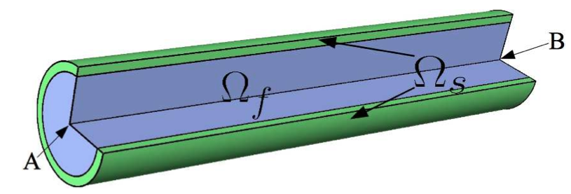
This represents the domains into the initial condition, with \(\Omega_f\) and \(\Omega_s\) respectively the fluid and the solid domain. The cylinder radius equals to \(r+\epsilon\), where \(r\) is the radius of the fluid domain and \(\epsilon\) the part of the solid domain.
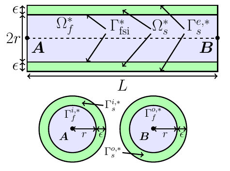
\(\Gamma^*_{fsi}\) is the interface between the fluid and solid domains, whereas \(\Gamma^{e,*}_s\) is the interface between the solid domain and the exterior. \(\Gamma_f^{i,*}\) and \(\Gamma_f^{o,*}\) are respectively the inflow and the outflow of the fluid domain. Likewise, \(\Gamma_s^{i,*}\) and \(\Gamma_s^{o,*}\) are the extremities of the solid domain.
During this benchmark, we will study two different cases, named BC-1 and BC-2, that differ from boundary conditions. BC-2 are conditions imposed to be more physiological than the ones from BC-1. So we waiting for more realistics based results from BC-2.
1.1. Boundary conditions
-
on \(\Gamma_f^{i,*}\) the pressure wave pulse \[ \boldsymbol{\sigma}_{f} \boldsymbol{n}_f = \left\{ \begin{aligned} & \left(-\frac{1.3332 \cdot 10^4}{2} \left( 1 - \cos \left( \frac{ \pi t} {1.5 \cdot 10^{-3}} \right) \right), 0 \right)^T \quad & \text{ if } t < 0.003 \\ & \boldsymbol{0} \quad & \text{ else } \end{aligned} \right. \]
-
We add the coupling conditions on \(\Gamma^*_{fsi}\)
Then we have two different cases :
-
Case BC-1
-
on \(\Gamma_f^{o,*}\) : \(\boldsymbol{\sigma}_{f} \boldsymbol{n}_f =0\)
-
on \(\Gamma_s^{i,*} \cup \Gamma_s^{o,*}\) a null displacement : \(\boldsymbol{\eta}_s=0\)
-
on \(\Gamma^{e,*}_{s}\) : \(\boldsymbol{F}_s\boldsymbol{\Sigma}_s\boldsymbol{n}_s^*=0\)
-
on \(\Gamma_f^{i,*}U \Gamma_f^{o,*}\) : \(\mathcal{A}^t_f=\boldsymbol{\mathrm{x}}^*\)
-
-
Case BC-2
-
on \(\Gamma_f^{o,*}\) : \(\boldsymbol{\sigma}_{f} \boldsymbol{n}_f = -P_0\boldsymbol{n}_f\)
-
on \(\Gamma_s^{i,*}\) a null displacement \(\boldsymbol{\eta}_s=0\)
-
on \(\Gamma^{e,*}_{s}\) : \(\boldsymbol{F}_s\boldsymbol{\Sigma}_s\boldsymbol{n}_s^* + \alpha \boldsymbol{\eta}_s=0\)
-
on \(\Gamma^{o,*}_{s}\) : \(\boldsymbol{F}_s\boldsymbol{\Sigma}_s\boldsymbol{n}_s^* =0\)
-
on \(\Gamma_f^{i,*}\) : \(\mathcal{A}^t_f=\boldsymbol{\mathrm{x}}^*\)
-
on \(\Gamma_f^{o,*}\) : \(\nabla \mathcal{A}^t_f \boldsymbol{n}_f^*=\boldsymbol{n}_f^*\)
-
2. Inputs
| Name | Description | Nominal Value | Units |
|---|---|---|---|
\(E_s\) |
Young’s modulus |
\(3 \times 10^6 \) |
\(dynes.cm^{-2}\) |
\(\nu_s\) |
Poisson’s ratio |
\(0.3\) |
dimensionless |
\(r\) |
fluid tube radius |
0.5 |
\(cm\) |
\(\epsilon\) |
solid tube radius |
0.1 |
\(cm\) |
\(L\) |
tube length |
5 |
\(cm\) |
\(A\) |
A coordinates |
(0,0,0) |
\(cm\) |
\(B\) |
B coordinates |
(5,0,0) |
\(cm\) |
\(\mu_f\) |
viscosity |
\(0.03\) |
\(poise\) |
\(\rho_f\) |
density |
\(1\) |
\(g.cm^{-3}\) |
\(R_p\) |
proximal resistance |
\(400\) |
|
\(R_d\) |
distal resistance |
\(6.2 \times 10^3\) |
|
\(C_d\) |
capacitance |
\(2.72 \times 10^{-4}\) |
3. Outputs
After solving the fluid struture model, we obtain \((\mathcal{A}^t, \boldsymbol{u}_f, p_f, \boldsymbol{\eta}_s)\)
with \(\mathcal{A}^t\) the ALE map, \(\boldsymbol{u}_f\) the fluid velocity, \(p_f\) the fluid pressure and \(\boldsymbol\eta_s\) the structure displacement.
4. Discretization
Here are the different configurations we worked on.
The parameter Incomp defines if we use the incompressibility constraint or not.
Config |
Fluid |
Structure |
|||||||
\(N_{elt}\) |
\(N_{geo}\) |
\(N_{dof}\) |
\(N_{elt}\) |
\(N_{geo}\) |
\(N_{dof}\) |
Incomp |
|||
\((1)\) |
\(13625\) |
\(1~(P2P1)\) |
\(69836\) |
\(12961\) |
\(1\) |
\(12876~(P1)\) |
No |
||
\((2)\) |
\(13625\) |
\(1~(P2P1)\) |
\(69836\) |
\(12961\) |
\(1\) |
\(81536~(P1)\) |
Yes |
||
\((3)\) |
\(1609\) |
\(2~(P3P2)\) |
\(30744\) |
\(3361\) |
\(2\) |
\(19878~(P2)\) |
No |
||
For the structure time discretization, we will use Newmark-beta method, with parameters \(\gamma=0.5\) and \(\beta=0.25\).
And for the fluid time discretization, BDF, at order \(2\), is the method we choose.
These two methods can be found in [Chabannes] papers.