 .pdf
.pdf
Stokes Boundary Layer Benchmark
Analysis Type: Oscillatory motion of viscous boundary layer
| this benchmark has been published by NAFEMS, it has not yet been implemented/tested using Feel++ |
1. Introduction
The Stokes oscillating plate case is one of the few transient flow examples that offer a closed-form solution for laminar flow over a smooth solid wall. The fluid motion, which is stimulated by an oscillating boundary, is dominated by viscous forces. It can be shown that the system of transport equations is reduced to a diffusion equation for a single velocity component [1,2] The integration of the diffusion equation over a longer time interval shall expose numerical diffusion of the applied spatial and temporal discretisation.
2. Objectives
Examine the accuracy of transient solver and the extent of false, numerical diffusion by comparing the velocity distribution throughout the simulation time interval with the analytical solution. The numerical error is manifested by the accelerated velocity decay and the phase shift of the oscillatory motion.
3. Geometry
-
Length of the simulation domain \((\mathrm{H} 6)\) is \(8.0 \mathrm{m}\)
-
Domain height (V7) is 5.0 \(\mathrm{m}\)
-
Domain width \(0.2 \mathrm{m}\) (although not important due to the case twodimensionality).
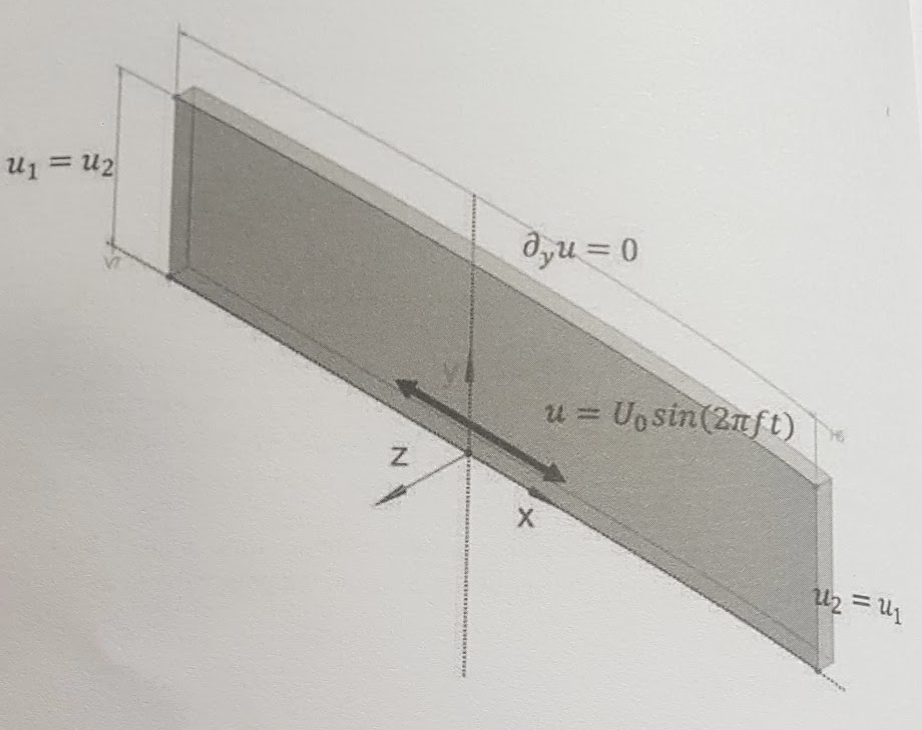
4. Case Definition
Sinusoidal oscillations in the \(x\) -direction are forced by prescribing a plate velocity function \(u=U_{0} \sin (2 \pi f t)\) to the bottom surface where:
-
\(U_{0}\) is the velocity amplitude set to \(1.0 \mathrm{m} / \mathrm{s}\)
-
\(f\) is the forced oscillation frequency set to \(1.0 \mathrm{Hz}\)
-
\(t\) is time.
5. Fluid Properties
Propagation of the low speed oscillatory motion depends solely on kinematic viscosity of the fluid:
-
\(v\) is kinematic viscosity of \(1.0 \mathrm{m}^{2} / \mathrm{s}\) (comparable to glycerol).
6. Initial Conditions
Zero velocity ( \(u\) ) and relative pressure ( \(p_{r e l}\) ) for the whole domain.
7. Boundary Conditions
-
The bottom plate has a prescribed velocity
-
\(u=U_{0} \sin (2 \pi f t)\) with no slip boundary conditions.
-
At the top surface, slip boundary conditions shall be used.
-
The vertical \(Y-Z\) surfaces at \(x=x_{\min }\) and \(x_{m a x}\) have periodic boundary conditions
-
For the streamwise velocity \(\left(u_{1}=u_{2}\right)\) assigned to them.
-
For the vertical \(X\) -Y surfaces, the symmetry or equivalent conditions shall be used.
8. Output
The analytical solution is \(u=U_{0} e^{-k y} \sin (2 \pi f t-k y)\) where:
-
\(k=\sqrt{\pi f / v}\) is the wave number;
-
\(v\) is fluid kinematic viscosity.
The velocity distribution should be compared to the analytical solution at different heights \((y)\) in the simulation domain. The following elevations are advised: \(y=0.1,0.2,0.4,0.8\) and \(2.0 \mathrm{m}\)
Dissipation of the velocity amplitude relative to the analytical solution \(\left(u_{n u m} / u-1\right)\) as well its phase shift \((\Delta t)\) should be calculated. The smaller the velocity amplitude difference and the phase shift, the lower the numerical diffusion.