.pdf
.pdf
Benchmarking and validation
This page summarizes how Maxwell formulations are validated and links to the benchmark suites available in this module.
1. Validation strategy
We validate both accuracy and robustness with complementary benchmark families:
-
manufactured-solution checks for formulation consistency,
-
reference geometries with known trends or external solvers,
-
nonlinear benchmark cases stressing convergence and solver behavior.
3. Manufactured-solution check
For a convergence-oriented verification, we set \(\mu_{\mathrm{o}}=1\) and prescribe an exact solution.
Given a sinusoidal exact field, we build the right-hand side and enforce exact Dirichlet boundary conditions:
\begin{aligned} \mathbf{J}&= \begin{pmatrix} 3 \pi^3 \cos(\pi x) \sin(\pi y)\sin(\pi z) \\ -6\pi^3 \sin(\pi x) \cos(\pi y) \sin(\pi z) \\ 3\pi^3 \sin(\pi x) \sin(\pi y) \cos(\pi z) \end{pmatrix} \\ \mathbf{A}_{exact}&=\begin{pmatrix} \pi \cos(\pi x) \sin(\pi y) \sin(\pi z)\\ -2\pi \sin(\pi x) \cos(\pi y) \sin(\pi z) \\ \pi \sin(\pi x) \sin(\pi y) \cos(\pi z)\end{pmatrix} \\ \mathbf{c}&=\begin{pmatrix}3 \pi^2 \cos(\pi z) \cos(\pi y)\sin(\pi x)\\0 \\-(3\pi^2) \sin(\pi z) \cos(\pi y)\cos(\pi x )\end{pmatrix} \end{aligned}
3.1. Regularized point system
\begin{aligned} \nabla \times \left(\frac{1}{\mu_{\mathrm{o}}} \nabla \times \mathbf{A} \right) + \epsilon \mathbf{A} &= \mathbf{J} \quad \text{ in } \Omega \\ \left.\mathbf{A}\right|_{\partial \Omega} &= \mathbf{A}_{exact} \end{aligned}
3.2. Saddle-point system
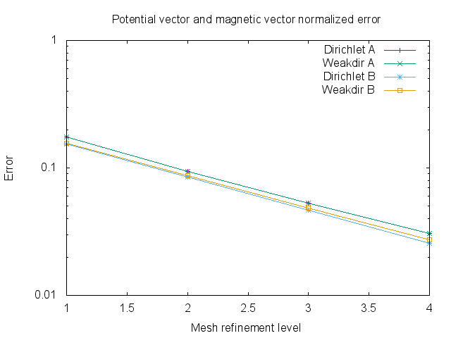
\begin{aligned} \nabla \times \left(\frac{1}{\mu_{\mathrm{o}}} \nabla \times \mathbf{A} \right) + \nabla p &= \mathbf{J} \quad \text{ in } \Omega \\ \nabla \cdot \mathbf{A} &= 0 \quad \text{ in } \Omega \\ \left.\mathbf{A}\right|_{\partial \Omega} &= \mathbf{A}_{exact} \\ \left.p\right|_{\partial \Omega} &= 0 \end{aligned}
The boundary condition can be applied with penalization or elimination. We compare both results: