Mixed Form Cahn-Hilliard PDE Model in 2D and 3D

1. Introduction

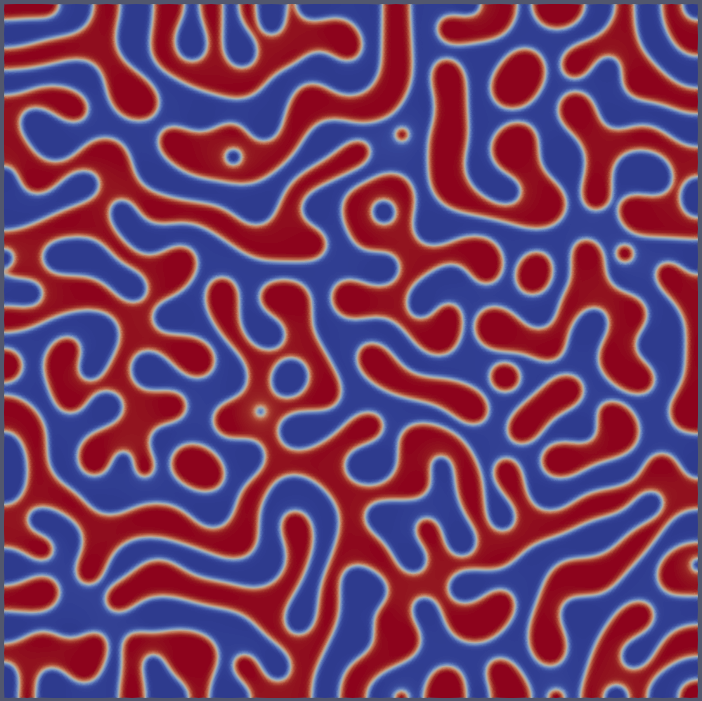
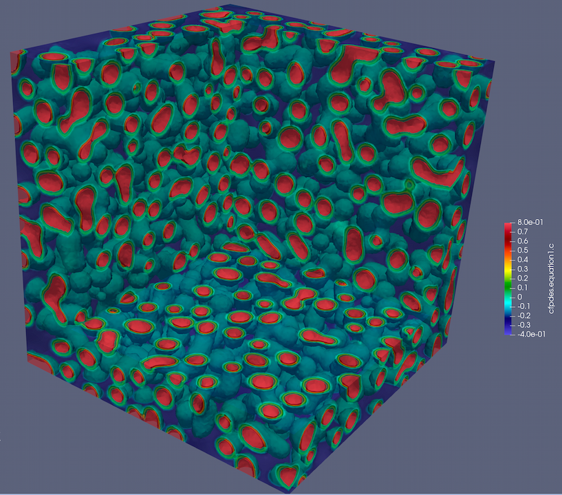
The Cahn-Hilliard equation is typically used to model phase separation in binary mixtures. In its mixed form, it is transformed into two coupled second-order equations to avoid dealing with fourth-order spatial derivatives directly. It was first introduced in the late 1950s by John W. Cahn and John E. Hilliard as a phenomenological model for spinodal decomposition - the spontaneous separation of a solution into multiple phases.

In a practical context, this equation can be used to study the evolution of microstructures in alloys, phase separation in polymers, or domain formation in thin magnetic films. It models the migration of atoms or particles driven by gradients of chemical potential, with the goal of minimizing the free energy of the system.

2. Features of the Cahn-Hilliard Equation

The Cahn-Hilliard equation possesses several key features that are crucial to its application in modeling phase separation processes:

It involves first-order time derivatives, and second- and fourth-order spatial derivatives. This reflects the interplay between diffusive transport (second order) and interface or surface tension effects (fourth order). The high order of the equation can make it difficult to solve numerically.
The mixed form of the Cahn-Hilliard equation involves two coupled second-order equations, making it more amenable to solution via standard finite element methods.
The equation involves a free energy density, which typically exhibits a double-well potential. This reflects the energetics of the two phases in a binary mixture. The double-well potential makes the problem nonlinear and may lead to "phase separation", i.e., regions where the concentration is close to either one of the minima of the potential.

3. Parameters in the Cahn-Hilliard Equation

The parameters involved in the Cahn-Hilliard equation have physical meanings:

The variable \(c\) stands for the concentration of one of the components.
The parameter \(M\) represents the mobility, which describes how fast particles or atoms can move.
The parameter \(\lambda\) is a gradient energy coefficient, accounting for energy associated with composition gradients.
The function \(f(c)\) is the bulk free energy density, which is minimized by the system.

In the mixed form of the Cahn-Hilliard equation, an additional field \(\mu\) is introduced. This is a chemical potential, which drives the evolution of the concentration field \(c\).

4. Mathematical Formulation

The mixed form of the Cahn-Hilliard equations in 2D and 3D is given by:

\[\begin{align*} \frac{\partial c}{\partial t} - \nabla \cdot M \nabla\mu &= 0 \quad {\rm in} \ \Omega, \\ \mu - \frac{d f}{d c} + \lambda \nabla^{2}c &= 0 \quad {\rm in} \ \Omega. \end{align*}\]

where \(c(\mathbf{x}, t)\) and \(\mu(\mathbf{x}, t)\) are the unknown fields at position \(\mathbf{x}\) and time \(t\), \(f(c)\) is usually a non-convex function of \(c\) (a fourth-order polynomial is commonly used), \(M\) is a scalar parameter, and \(\lambda\) is a gradient energy coefficient.

The weak form of the problem reads: find (\(c, \mu\)) in \(V \times V\) such that

\[\begin{align*} \int_{\Omega} \frac{\partial c}{\partial t} q \, {\rm d} x + \int_{\Omega} M \nabla\mu \cdot \nabla q \, {\rm d} x &= 0 \quad \forall \ q \in V, \\ \int_{\Omega} \mu v \, {\rm d} x - \int_{\Omega} \frac{d f}{d c} v \, {\rm d} x - \int_{\Omega} \lambda \nabla c \cdot \nabla v \, {\rm d} x &= 0 \quad \forall \ v \in V. \end{align*}\]

5. Problem Specification

Geometry: A unit square for 2D or a unit cube for 3D.
Initial condition: A small random perturbation around \(c = 0.5\).
Free energy function: \(f(c) = c^2 (c^2 - 1)\), corresponding to a double-well potential.
Mobility: \(M = 1\).
Gradient energy coefficient: \(\lambda = 0.01\).
Boundary conditions: as per the mathematical formulation.

6. Numerical Scheme

A finite element method is used to discretize the PDEs using the Feel++ coefficient form pde toolbox.

7. Input Data

For our benchmark, we will consider the following:

Mobility: \(M = 1\)
Gradient energy coefficient: \(\lambda = 0.01\).
Domain: a unit square or cube with grid size \(\Delta x = 0.01\).
Time: from \(t = 0\) to \(t = 1\) with a time step of \(\Delta t = 0.001\).
Initial concentration: a small random perturbation around \(c = 0.5\).

Json data file for coefficient form pde toolbox

"Models":
{
  "cfpdes":{ "equations":["equation1","equation2"] },
  "equation1":{
    "setup":{
        "unknown":{"basis":"Pch1","name":"c","symbol":"c"},
        "coefficients":{
           "d": "1",
           "gamma": "{-equation2_grad_mu_0,-equation2_grad_mu_1,-equation2_grad_mu_2}"
  }}},
  "equation2":{
    "setup":{
        "unknown":{"basis":"Pch1","name":"mu","symbol":"mu"},
        "coefficients":{
           "gamma":"{lambda*equation1_grad_c_0,lambda*equation1_grad_c_1, lambda*equation1_grad_c_2}",
           "a":"1",
           "f": "equation1_c^2*(equation1_c^2 - 1)"
  } } }
}

8. Results

The following figures show the evolution of the concentration field \(c\) and the chemical potential \(\mu\) in 2D and 3D.

8.1. 2D Results

Figure 1. 2D

8.2. 3D results

Figure 2. 3D (t = 6e-3s)