 .pdf
.pdf
Thermal bridges in building construction
1. Context
ISO 10211:2007 sets out the specifications for a three-dimensional and a two-dimensional geometrical model of a thermal bridge for the numerical calculation of:
-
heat flows, in order to assess the overall heat loss from a building or part of it;
-
minimum surface temperatures, in order to assess the risk of surface condensation.
These specifications include the geometrical boundaries and subdivisions of the model, the thermal boundary conditions, and the thermal values and relationships to be used.
ISO 10211:2007 is based upon the following assumptions:
-
all physical properties are independent of temperature;
-
there are no heat sources within the building element.
ISO 10211:2007 can also be used for the derivation of linear and point thermal transmittances and of surface temperature factors. More information here.
2. Parameters
The parameters for this benchmark case are given by:
{
  "Parameters": {
    "h_top": "1.0/0.06",
    "h_bottom": "1.0/0.11",
    "T0_top": 0,
    "T0_bottom": 20
  }
}
These parameters define the top and bottom heat transfer coefficients (h_top and h_bottom) and the exterior temperatures (T0_top and T0_bottom).
3. Geometry and Mesh
This case uses the following mesh configuration:
{
  "Meshes": {
    "heat": {
      "Import": {
        "filename": "$cfgdir/case2.geo",
        "hsize": 0.001
      }
    }
  }
}
The geometry is defined in the case2.geo file, with a mesh size of 0.001.
4. Materials
The materials used in the model include concrete, wood, insulation, and aluminum. The specific parameters are:
{
  "Materials": {
    // material data here
  }
}
Each material has specific properties including thermal conductivity (k), specific heat capacity (Cp), and density (rho).
5. Mathematical Formulation
This simulation solves the steady state heat equation which can be represented by the partial differential equation (PDE):
where:
-
T is the temperature,
-
k is the thermal conductivity.
6. Boundary Conditions
The boundary conditions define the state of heat at the boundaries of the geometry.
{
  "BoundaryConditions": {
    // boundary condition data here
  }
}
The boundary conditions are given by a convective heat flux on the top and bottom of the model. The associated mathematical expressions are:
- For the top
- For the bottom
where:
-
h is the heat transfer coefficient,
-
T is the temperature,
-
T0 is the exterior temperature,
-
q_n is the heat flux normal to the boundary.
7. Post-processing
The post-processing step includes the extraction and analysis of data:
{
  "PostProcess": {
    // post-processing data here
  }
}
In the post-processing stage, several quantities are computed, including temperature fields, normal heat flux, and the heat flux at specific points.
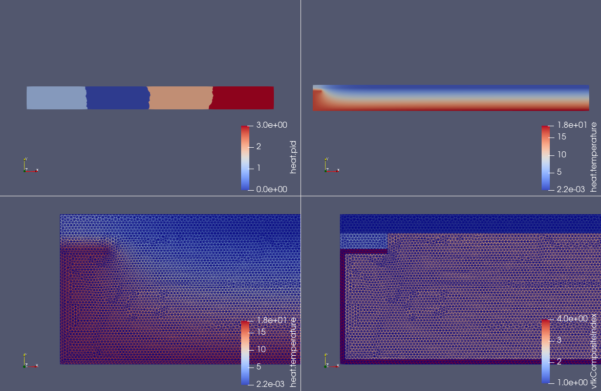
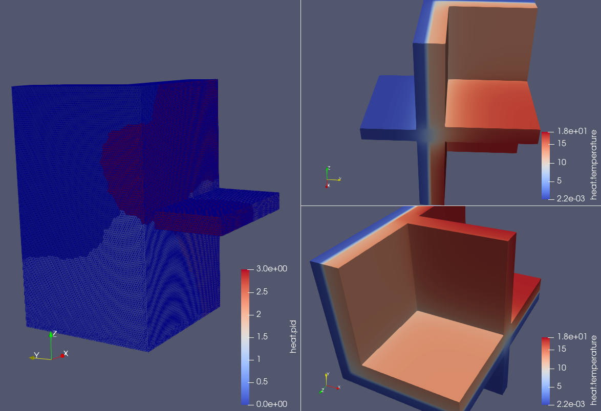
8. Results
Here, we present the results from the simulation.
9. Running the model
The configuration file is in Building/ThermalBridgesENISO10211/case2.cfg.
The command line in feelpp-toolboxes docker or singularity reads
$ mpirun -np 4 feelpp_toolbox_heat --config-file case2.cfg$ mpirun -np 4 feelpp_toolbox_heat --config-file case3.cfg