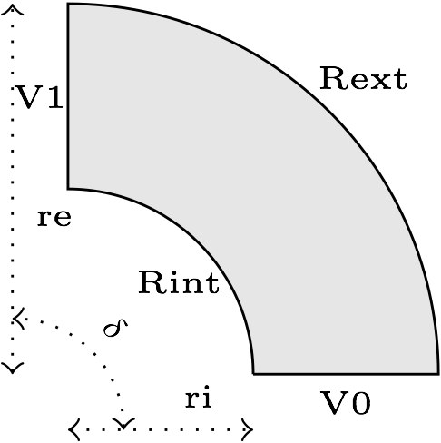
Quarter-Turn
In this example, we will estimate the current distribution in a stranded conductor. An electrical potential \(V_0\) is applied to the entry/exit of the conductor.
1. Running the case
The command line to run this case in 2D is
mpirun -np 4 feelpp_toolbox_electric --case "github:{path:toolboxes/electric/cases/quarter-turn}" --case.config-file 2d.cfg--case "github:{path:toolboxes/electric/cases/quarter-turn}"
--case.config-file 2d.cfg
The command line to run this case in 3D is
mpirun -np 4 feelpp_toolbox_electric --case "github:{path:toolboxes/electric/cases/quarter-turn}" --case.config-file 3d.cfg--case "github:{path:toolboxes/electric/cases/quarter-turn}"
--case.config-file 3d.cfg
2. Geometry
The conductor consists in a rectangular cross section torus which is somehow "cut" to allow for applying electrical potential.+
In 2D, the geometry is as follow:

In 3D, this is the same geometry, but extruded along the z axis.
3. Input parameters
| Name | Description | Value | Unit | |
|---|---|---|---|---|
\(r_i\) |
internal radius |
1 |
\(m\) |
|
\(r_e\) |
external radius |
2 |
\(m\) |
|
\(\delta\) |
angle |
\(\pi/2\) |
\(rad\) |
|
\(V_D\) |
electrical potential |
9 |
\(V\) |
3.1. Model & Toolbox
-
This problem is described by a steady electric conduction model for the potential \(V\).
-
toolbox: electric
3.2. Materials
| Name | Description | Marker | Value | Unit | |
|---|---|---|---|---|---|
\(\sigma\) |
electric conductivity |
omega |
\(4.8e7\) |
\(S.m^{-1}\) |
3.3. Boundary conditions
The boundary conditions are imposed electric potential on entry/exit (V0, V1).
On the other boundaries, zero normal current is applied through the natural homogeneous Neumann condition.
| Marker | Type | Value | |
|---|---|---|---|
V0 |
Dirichlet |
0 |
|
V1 |
Dirichlet |
\(V_D\) |
|
Rint, Rext, top*, bottom* |
Neumann |
0 |
*: only in 3D
4. Outputs
The main fields of concern are:
-
electric potential \(V\)
-
current density \(\mathbf{j}\)
-
electric field \(\mathbf{E}\)
-
Joule losses density
5. Verification Benchmark
The analytical solution is given by:
We will check if the approximations converge at the appropriate rate:
-
k+1 for the \(L_2\) norm for \(V\)
-
k for the \(H_1\) norm for \(V\)
-
k for the \(L_2\) norm for \(\mathbf{E}\) and \(\mathbf{j}\)
-
k-1 for the \(H_1\) norm for \(\mathbf{E}\) and \(\mathbf{j}\)
 .pdf
.pdf