.pdf
.pdf
2D Advection-diffusion with Taylor-Green Vortex
This page can be downloaded as a pdf file or as a Jupyter notebook file by clicking on the corresponding icons in the toolbar. It exemplifies the usage of the Coefficient form PDE toolbox in Python.
1. Introduction
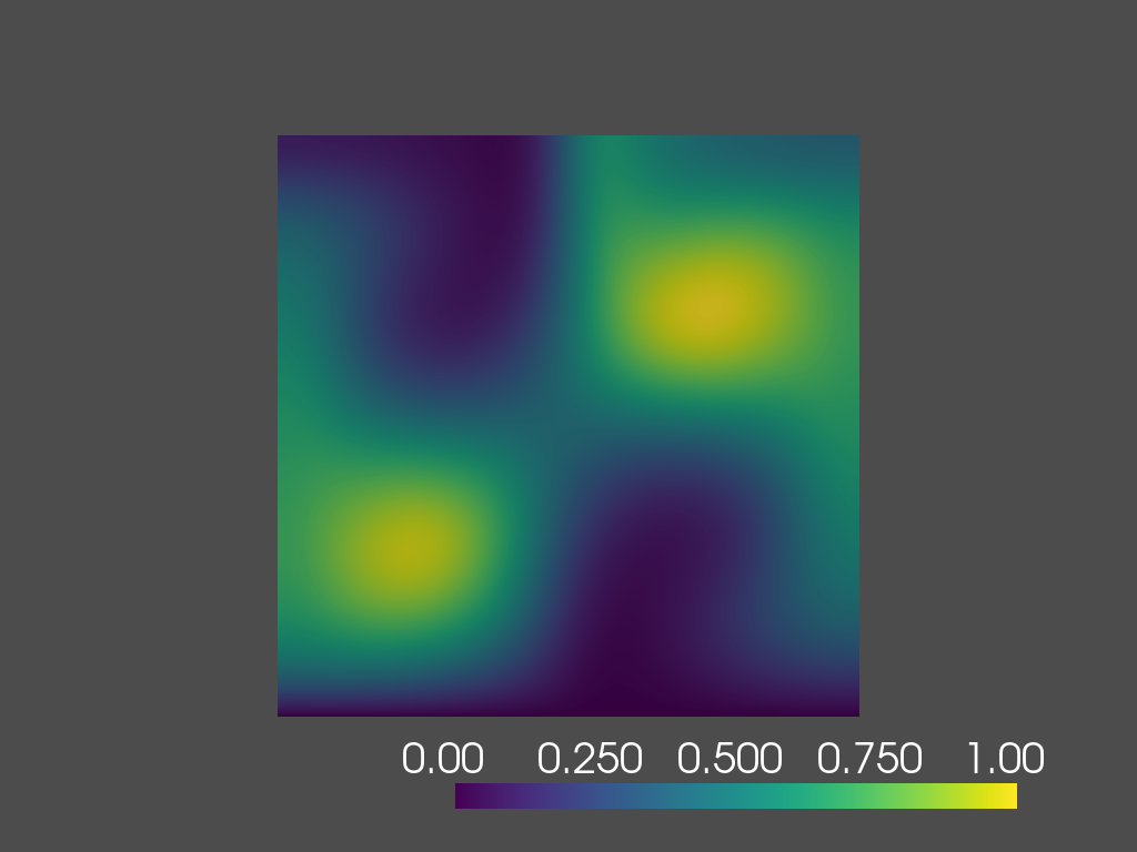
We study the solution of a 2D advection-diffusion equation (used to model the dispersion of a contaminant) in presence of a Taylor-Green vortex \(\beta(x,t)\). The problem can be solved for different values of the diffusion coefficient \(\mu\).
2. Advection-diffusion with Taylor-Green Vortex
The problem is defined on the spatial domain \(\Omega = (-1, 1)^2\) with Dirichlet boundary \(\Gamma_D := (-1, 1) \times \{-1\}\) and Neumann boundary \(\Gamma_N := \partial\Omega \setminus \Gamma_D\). The governing parametric PDE (pPDE) can be described as follows:
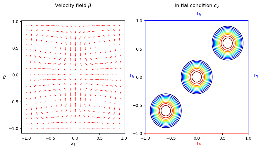
Where, the velocity field \(\beta := (\sin(\pi x_1) \cos(\pi x_2), -\cos(\pi x_1) \sin(\pi x_2))^{\top}\), \(x = (x_1, x_2)\), is a solenoidal field. The initial condition, \(c_0(\cdot; \mu): \Omega \rightarrow \mathbb{R}\), is given by the sum of three Wendland functions \(\bar{\psi}_{2,1}^i\) of radius 0.4 and centers located at \((-0.6, -0.6)\), \((0, 0)\) and \((0.6, 0.6)\). The Wendland functions are radial functions with compact support on the unit ball, and \(\psi_{2,1}(r)\) has the following closed form
Appropriate transformations have been applied to \(\psi_{2,1}(r)\) in order to get the scaled and translated Wendland functions \(\bar{\psi}_{2,1}^i\).
The velocity field \(\beta\), the initial condition \(c_0(\cdot; \mu)\), and the boundaries are illustrated in the following figure.
3. Configuring the simulation
3.1. Setting up the Feel++ Environment
To set up the Feel++ environment, we create an environment and set the associated repository for the results.
import sys
import feelpp
import feelpp.toolboxes.core as tb
from feelpp.toolboxes.cfpdes import *

sys.argv = ["feelpp_cfpdes_Taylor_Green"]
e = feelpp.Environment(sys.argv,
                        opts=tb.toolboxes_options("coefficient-form-pdes", "cfpdes"),
                        config=feelpp.globalRepository("cfpdes-Taylor_Green"))
Results
[ Starting Feel++ ] application feelpp_cfpdes_Taylor_Green
 . feelpp_cfpdes_Taylor_Green files are stored in /home/feelppdb/cfpdes-Taylor_Green/np_1
 .. logfiles :/home/feelppdb/cfpdes-Taylor_Green/np_1/logs
3.2. Geometry and Mesh
We will construct a geometric domain for our Finite Element Model.
In the 2D case, the domain is a square with side lengths of 2 units, centered at the origin, and can be represented as [-1,1]2
. The bottom edge is designated as the Dirichlet boundary (\(\Gamma_D\)), while the left, top, and right edges form the Neumann boundary (\(\Gamma_N\)).
We propose also the creation of a 3D case, where the domain is the cube [-1,1]3. One face of the cube is assigned as the Dirichlet boundary (\(\Gamma_D\)), and the rest of the faces form the Neumann boundary (\(\Gamma_N\)).
Both the 2D and 3D geometries allow for customization of mesh sizes.
def generateGeometry(filename, dim=2, hsize=0.1):
    """create gmsh mesh

    Args:
        filename (str): name of the file
        dim (int): dimension of the mesh
        hsize (float): mesh size
    """
    geo = """SetFactory("OpenCASCADE");
    h = {};
    dim = {};
    """.format(hsize, dim)
    if dim == 2:
        geo += """
        Rectangle(1) = {-1, -1, 0, 2, 2, 0};
        Characteristic Length{ PointsOf{ Surface{1}; } } = h;
        Physical Curve("Gamma_D") = {1};
        Physical Curve("Gamma_N") = {2,3,4};
        Physical Surface("Omega") = {1};
        """
    elif dim == 3:
        geo += """
        Box(1) = {-1, -1, -1, 2, 2, 2};
        Characteristic Length{ PointsOf{ Volume{1}; } } = h;
        Physical Surface("Gamma_D") = {5};
        Physical Surface("Gamma_N") = {1,2,3,4,6};
        Physical Volume("Omega") = {1};
        """
    with open(filename, 'w') as f:
        # Write the string to the file
        f.write(geo)

def getMesh(filename, hsize=0.05, dim=2, verbose=False):
    """create mesh

    Args:
        filename (str): name of the file
        hsize (float): mesh size
        dim (int): dimension of the mesh
        verbose (bool): verbose mode
    """
    import os
    for ext in [".msh",".geo"]:
        f = os.path.splitext(filename)[0] + ext
        if os.path.exists(f):
            os.remove(f)
    if verbose:
        print(f"generate mesh {filename} with hsize={hsize} and dimension={dim}")
    generateGeometry(filename=filename, dim=dim, hsize=hsize)
    mesh = feelpp.load(feelpp.mesh(dim=dim, realdim=dim), filename, hsize)
    return mesh
3.3. Defining Model Properties
The next step is to define the model properties. We achieve this by creating a JSON file containing the following information:
-
The PDE coefficients, which follow the format: \(d \frac{\partial u}{\partial t} + \nabla \cdot (-c \nabla u - \alpha u + \gamma) + \beta \cdot \nabla u + a u = f\), more details about the coefficients can be found in the CFPDEs documentation.
-
The approximation space (e.g., continuous piecewise polynomial finite elements \(P^k \text{ for } k=0,1,2\))
-
Domain and boundary conditions, using the markers defined previously in the geometry file.
-
Initial condition
-
Post-processing (e.g., exporting the solution, computing the error, …)
More details about modelling using JSON files can be found in the JSON documentation.
In the following code, we created a lambda function called Taylor_Green_json to generate the JSON file depending on the polynomial order k and the diffusion coefficient \(\mu=\frac{1}{Pe}\).
Taylor_Green_json = lambda order,dim=2,mu=(1/30),name="c":  {
    "Name": "Taylor_Green",
    "ShortName": "Taylor_Green",
    "Models":
    {
        f"cfpdes-{dim}d":
        {
            "equations":"AdvDiff"
        },
        "AdvDiff":{
            "setup":{
                "unknown":{
                    "basis":f"Pch{order}",
                    "name":f"{name}",
                    "symbol":"c"
                },
                "coefficients":{
                    "d":"1.",
                    "c":f"{mu}",
                    "beta":"{sin(pi*x)*cos(pi*y),-cos(pi*x)*sin(pi*y)}:x:y" if dim==2 else "{sin(pi*x)*cos(pi*y)*cos(pi*z),-0.5*cos(pi*x)*sin(pi*y)*cos(pi*z),-0.5*cos(pi*x)*cos(pi*y)*sin(pi*z)}:x:y:z",
                    "f":"0."
                }
            }
        }
    },

    "Materials":
    {
        "Omega":
        {
            "markers":["Omega"]
        }
    },
    "BoundaryConditions":
    {
        "AdvDiff":
        {
            "Dirichlet":
            {
                "g":
                {
                    "markers":["Gamma_D"],
                    "expr":"0"
                }
            },
            "Neumann":{
                "m":
                {
                    "markers":["Gamma_N"],
                    "expr":"0"
                }
            }
        }
    },
    "InitialConditions":
    {
        "AdvDiff":
        {
            f"{name}":
            {
                "Expression":
                {
                    "wendland":
                    {
                        "markers":["Omega"],
                        "expr":"((1-2.5*sqrt((x+0.6)^2+(y+0.6)^2))>0)*(1-2.5*sqrt((x+0.6)^2+(y+0.6)^2))^3*(3*(2.5*sqrt((x+0.6)^2+(y+0.6)^2))+1)+((1-2.5*sqrt((x)^2+(y)^2))>0)*(1-2.5*sqrt((x)^2+(y)^2))^3*(3*(2.5*sqrt((x)^2+(y)^2))+1)+((1-2.5*sqrt((x-0.6)^2+(y-0.6)^2))>0)*(1-2.5*sqrt((x-0.6)^2+(y-0.6)^2))^3*(3*(2.5*sqrt((x-0.6)^2+(y-0.6)^2))+1):x:y" if dim==2 else "((1-2.5*sqrt((x+0.6)^2+(y+0.6)^2+(z+0.6)^2))>0)*(1-2.5*sqrt((x+0.6)^2+(y+0.6)^2+(z+0.6)^2))^3*(3*(2.5*sqrt((x+0.6)^2+(y+0.6)^2+(z+0.6)^2))+1)+((1-2.5*sqrt((x)^2+(y)^2+(z)^2))>0)*(1-2.5*sqrt((x)^2+(y)^2+(z)^2))^3*(3*(2.5*sqrt((x)^2+(y)^2+(z)^2))+1)+((1-2.5*sqrt((x-0.6)^2+(y-0.6)^2+(z-0.6)^2))>0)*(1-2.5*sqrt((x-0.6)^2+(y-0.6)^2+(z-0.6)^2))^3*(3*(2.5*sqrt((x-0.6)^2+(y-0.6)^2+(z-0.6)^2))+1):x:y:z"
                    }
                }
            }
        }
    },
    "PostProcess":
    {
        f"cfpdes-{dim}d":
        {
            "Exports":
            {
                "fields":["all"]
            }
        }
    }
}
3.3.1. Example: Using the JSON File
Let’s use the Taylor_Green_json function to generate a JSON file with specific parameters:
-
Polynomial order: 2
-
Dimension: 2
-
Mu: 1/30
Taylor_Green_json(order=2, dim=2, mu=1/30, name="c")Results
{'Name': 'Taylor_Green',
 'ShortName': 'Taylor_Green',
 'Models': {'cfpdes-2d': {'equations': 'AdvDiff'},
  'AdvDiff': {'setup': {'unknown': {'basis': 'Pch2',
     'name': 'c',
     'symbol': 'c'},
    'coefficients': {'d': '1.',
     'c': '0.03333333333333333',
     'beta': '{sin(pi*x)*cos(pi*y),-cos(pi*x)*sin(pi*y)}:x:y',
     'f': '0.'}}}},
 'Materials': {'Omega': {'markers': ['Omega']}},
 'BoundaryConditions': {'AdvDiff': {'Dirichlet': {'g': {'markers': ['Gamma_D'],
     'expr': '0'}},
   'Neumann': {'m': {'markers': ['Gamma_N'], 'expr': '0'}}}},
 'InitialConditions': {'AdvDiff': {'c': {'Expression': {'wendland': {'markers': ['Omega'],
      'expr': '((1-2.5*sqrt((x+0.6)^2+(y+0.6)^2))>0)*(1-2.5*sqrt((x+0.6)^2+(y+0.6)^2))^3*(3*(2.5*sqrt((x+0.6)^2+(y+0.6)^2))+1)+((1-2.5*sqrt((x)^2+(y)^2))>0)*(1-2.5*sqrt((x)^2+(y)^2))^3*(3*(2.5*sqrt((x)^2+(y)^2))+1)+((1-2.5*sqrt((x-0.6)^2+(y-0.6)^2))>0)*(1-2.5*sqrt((x-0.6)^2+(y-0.6)^2))^3*(3*(2.5*sqrt((x-0.6)^2+(y-0.6)^2))+1):x:y'}}}}},
 'PostProcess': {'cfpdes-2d': {'Exports': {'fields': ['all']}}}}
3.4. Time Scheme
The time scheme is defined in a .cfg file.
The Model CFG (.cfg) files allow to pass command line options to Feel++ applications. In particular, it allows to
-
setup the output directory
-
setup the mesh
-
setup the time scheme
-
define the solution strategy and configure the linear/non-linear algebraic solvers.
and other options that are specific to the toolbox being used.
For further details, see the CFG documentation.
Taylor_Green_cfg = lambda time_order=2, t0=0, T=0.2, dt=0.1: f"""
case.dimensions=2
[cfpdes]
#filename=$cfgdir/Taylor_Green.json
pc-type=gamg
ksp-converged-reason=
#verbose=1
#solver=Newton
snes-monitor=1
reuse-prec=1
#use-cst-matrix=0
#use-cst-vector=0
#snes-line-search-type=l2#basic
[cfpdes.AdvDiff]
#time-stepping=Theta
#stabilization=1
#stabilization.type=unusual-gls #supg#unusual-gls #gls
[cfpdes.AdvDiff.bdf]
order={time_order}

[ts]
time-initial={t0}
time-step={dt}
time-final={T}
restart.at-last-save=true
"""4. Solving the Problem and Exporting the Results
To solve the problem, we define a function called SolveTG which takes the mesh size, JSON and cfg files as inputs, initializes the problem (mesh, properties, and configuration), solves it iteratively for each time step, and exports the results.
def SolveTG(hsize, json, cfg, dim=2, verbose=False, measure=False):
    if verbose:
        print(f"Solving the Taylor green vortex advection-diffusion problem for hsize = {hsize}...")

    feelpp.Environment.setConfigFile(cfg)
    AdvDiff = cfpdes(dim=dim, keyword=f"cfpdes-{dim}d")
    AdvDiff.setMesh(getMesh(f"omega-{dim}d.geo", hsize=hsize, dim=dim, verbose=verbose))
    AdvDiff.setModelProperties(json)
    AdvDiff.init(buildModelAlgebraicFactory=True)
    AdvDiff.printAndSaveInfo()
    measures = []
    AdvDiff.startTimeStep()

    if AdvDiff.isStationary():
        AdvDiff.solve()
        AdvDiff.exportResults()
    else:
        while not AdvDiff.timeStepBase().isFinished():
            if AdvDiff.worldComm().isMasterRank():
                print("============================================================\n")
                print(f"time simulation: {AdvDiff.time()} s\n")
                print("============================================================\n")

            AdvDiff.solve()
            AdvDiff.exportResults()

            if measure:
                measures.append(AdvDiff.postProcessMeasures().values())
            AdvDiff.updateTimeStep()

    if measure:
        return measures
4.1. Example Usage
Now, let’s see an example of how to use the SolveTG function to solve the Taylor-Green Vortex problem with specific parameters.
-
0.04: Mesh size. -
order=2: Order of the polynomial used in the approximation space. -
dim=2: Dimension of the problem. -
mu=1/30: Value of the diffusion coefficient \(\mu\). -
"Taylor_Green.cfg": The name of the configuration file that we generated in the previous section.
SolveTG(0.04, Taylor_Green_json(order=2, dim=2, mu=1/30, name="c"), "Taylor_Green.cfg")|
The choice of the mesh size is not arbitrary and is based on the following criteria:
In our case, we have \(||\beta||_{L^\infty} = 1\) and \(\mu \in P := [1/50, 1/10\)]. Therefore, we need to choose \(h\) such that \(h \leq 0.04\). |
5. Visualizing the Results in the Notebook
Once the Taylor-Green Vortex problem is solved, it’s useful to visualize the results to gain insights into the behavior of the solution over time. In this section, we use pyvista library for visualization directly within the notebook. We will be displaying the solution at different time instances.
To run this visualization, you need to have the pyvista and xvfbwrapper Python packages installed.
|
import vtk
import pyvista as pv
import numpy as np
import os
try:
from xvfbwrapper import Xvfb
vdisplay = Xvfb()
vdisplay.start()
except:
print("Please install 'xvfbwrapper' Python package")
exit(0)
# Define the path to the case file directory
case_path = os.path.abspath("cfpdes-2d.exports/Export.case")
# Create the EnSight reader
reader = vtk.vtkEnSightGoldBinaryReader()
reader.SetCaseFileName(case_path)
reader.ReadAllVariablesOn()
reader.Update()
# Extract the number of time steps
num_time_steps = reader.GetTimeSets().GetItem(0).GetNumberOfTuples()
# Create the Plotter
plotter = pv.Plotter()
# Specify the desired time steps
desired_times = [0.2, 0.8, 1.4, 2.0, 2.0]
# Get the time values as a list
time_values = [reader.GetTimeSets().GetItem(0).GetValue(i) for i in range(num_time_steps)]
# Loop through the desired time steps
for time in desired_times:
closest_time = min(time_values, key=lambda x: abs(x - time))
# Set the reader's time step
reader.SetTimeValue(closest_time)
reader.Update()
# Convert the output to a PyVista mesh
mesh = pv.wrap(reader.GetOutput())
# Rescale the scalar data
block_id = 0
block = mesh[block_id]
scalars = block.point_data["cfpdes.AdvDiff.c"]
scalars /= np.max(np.abs(scalars))
# Add the rescaled mesh to the Plotter
plotter.add_mesh(block, scalars=scalars, cmap="viridis", show_edges=False)
plotter.view_xy()
# Show the plot
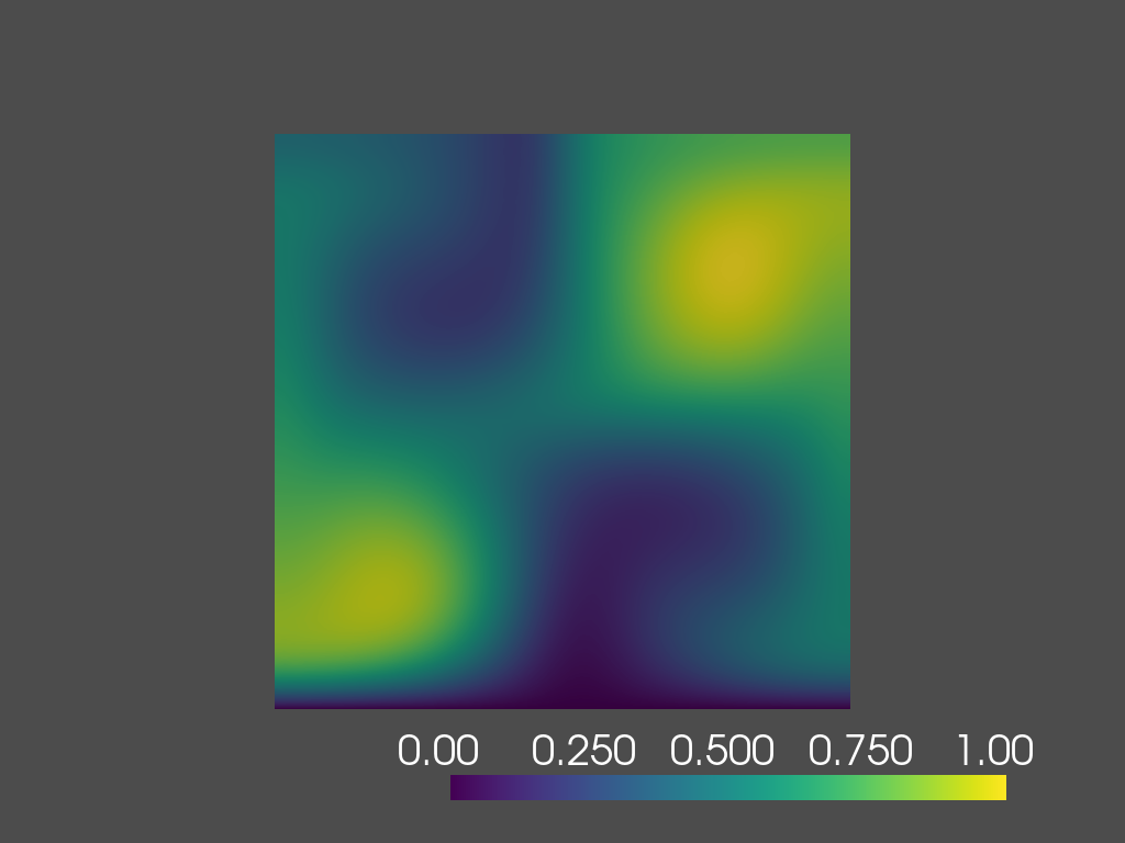
plotter.show()Results
time=0.2s
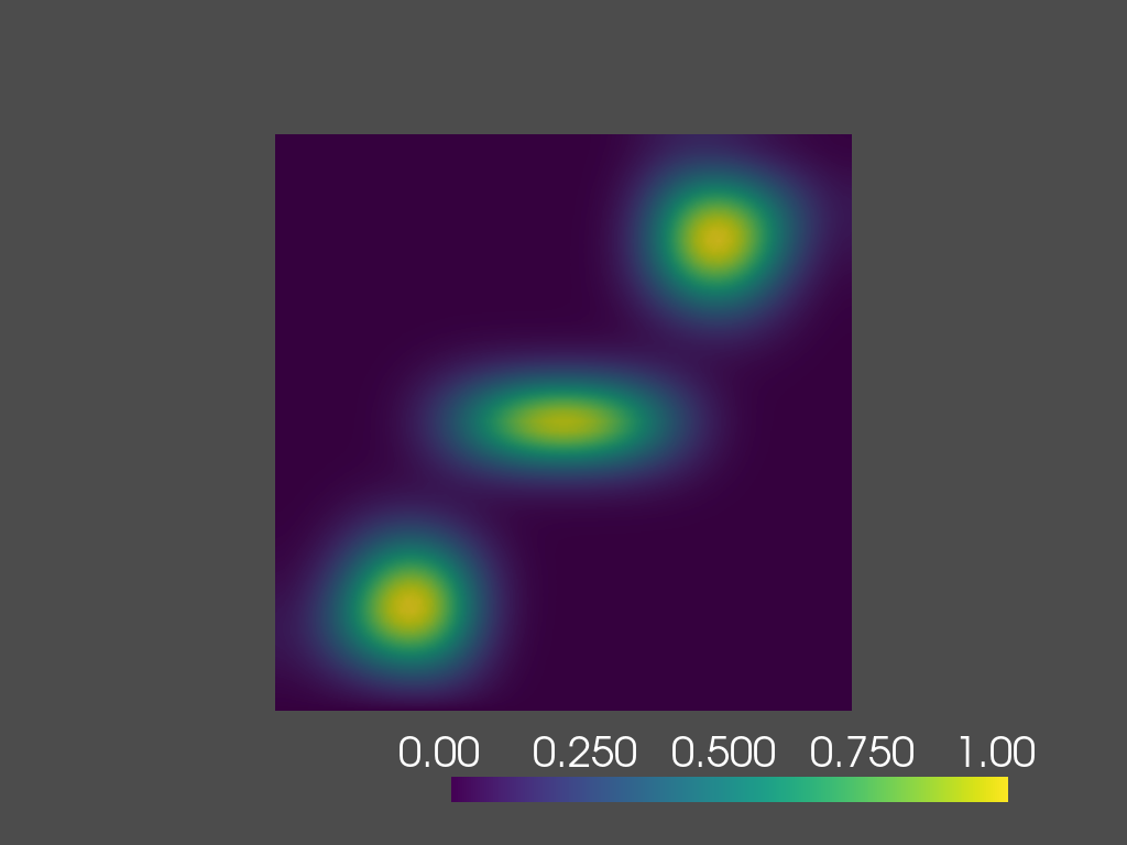
time=0.8s
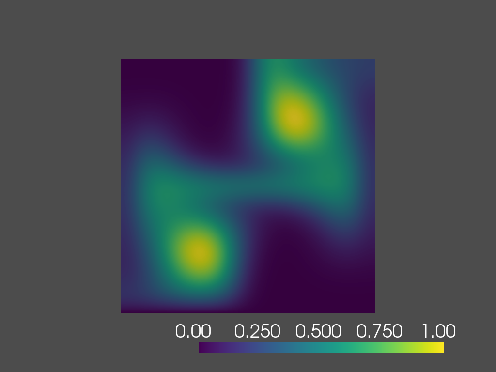
time=1.4s
time=2.0s