.pdf
.pdf
Drug Delivery in a Coronary Stent
We took this example from : [Socrates_Dokos_(auth.)]_Modelling_Organs,_Tissues(z-lib.org) .
1. Description
\(\quad\) In this example, we will build a drug delivery in a coronary stent model.
\(\quad\) A drug-eluting stent is used to re-open the vessel in a occuled artery for blood flow. This stent slowly release drugs to prevent scar tissue formation and keep the artery open. Typcally, we use pactitaxel or sirolimus and its analogues including everolimus. We wish to implement a simplified model of such a system to determine the blood drug distribution as a function of time along the artery. We have this PDE:
For the velocity, we have this profile:
where \(u\) is the velocity in the axial direction, \(u_{max}\) is the maximum velocity (=50 \(cm^{-1}\)), \(R\) is the arterial radius (=1mm), and r is the radial distance from the central axis.
We use a mono-exponential decay of stent drug-content:
\(\quad\) The duration in the example is \(10^5s\). But, we will only compute 1s duration and use a time step of \(1e^{-4}s\).
2. Input
We will use those inputs:
Name |
Description |
Values |
Units |
\(u_{max}\) |
Maximum blood velocity |
\(5 0\) |
\(cm/s\) |
\(D\) |
Drug diffusion coefficient |
\(2.56 \times 10^{-4}\) |
\(cm^{2}/ min\) |
\(k\) |
Drug release rate |
\(0.2\) |
\(1 / hour\) |
\(R\) |
Artery radius |
\(1\) |
\(mm\) |
\(L_{artery}\) |
Arterysegment lenght |
\(9\) |
\(mm\) |
\(L_{stent}\) |
Stent lenght |
\(6\) |
\(mm\) |
\(Mo\) |
Initial stent drug content |
\(49.2\) |
\(nmol\) |
After converting units, we obtain these values:
Name |
Description |
Values |
Units |
\(u_{max}\) |
Maximum blood velocity |
\(0.5\) |
\(m\ s^{-1}\) |
\(D\) |
Drug diffusion coefficient |
\(4.266 \times 10^{-10}\) |
\(m^{2}/ s\) |
\(k\) |
Drug release rate |
\(5.555\) |
\(1 / s\) |
\(R\) |
Artery radius |
\(1 \times 10^{-3}\) |
\(m\) |
\(L_{artery}\) |
Arterysegment lenght |
\(9 \times 10^{-3}\) |
\(m\) |
\(L_{stent}\) |
Stent lenght |
\(6 \times 10^{-3}\) |
\(m\) |
\(Mo\) |
Initial stent drug content |
\(49.2\times 10^{-9}\) |
\(mol\) |
3. Data files
The case data files are available in Github here
3.1. Json file
3.1.1. Names
A model JSON file starts by giving names (long and short).
"Name": "Drug Delivery in a Coronary Stent", (1)
"ShortName":"Stent",(2)
| 1 | Name of the example, usually printed on-screen and in log files during simulations |
| 2 | Short name of the example, it is used to create directories to store the results of the simulation of the model |
3.1.2. Parameters
As shown above, we have those parameters. Note that we use \(kr\) instead of \(k\) because we use the heat toolbox and k is used in heat PDE.
  "Parameters":
  {
    "umax": "0.5",
      "D":"4.266e-10",
     "R": "1e-3",
     "Mo":"49e-9",
     "kr":"5.555e-5",
     "lStent":"6e-3",
  }
3.1.3. Materials
This section of the Model JSON file defines material properties linking the Physical Entities in the mesh data structures to these properties.
  "Materials":
  {
    "Fluid":
      {
         "markers":"Fluid",
          "rho":"1.0",
          "mu":"0",
          "k":"D:D",
          "Cp":"1.0"
      }
  },
3.1.4. Boundary Conditions
This section of the Model JSON file defines the boundary conditions.
  "BoundaryConditions":
  {
      "temperature": (1)
      {
           "Dirichlet": (2)
          {
            "inflow": (3)
            {
              "expr":"0" (4)
            }
          },
          "Neumann": (2)
          {
            "stent": (3)
            {
              "expr":"kr*M/(2*pi*R*lStent):kr:M:lStent:R" (4)
            },
            "artery":(3)
            {
              "expr":"0" (4)
            },
            "outflow":(3)
            {
              "expr":"0"(4)
            }
          }
      }
},| 1 | the field name of the toolbox to which the boundary condition is associated |
| 2 | the type of boundary condition to apply |
| 3 | the physical entity (associated to the mesh) to which the condition is applied |
| 4 | the mathematical expression associated to the condition |
3.1.5. InInitial Conditions
"InitialConditions" : {
"temperature" : {
"" : {
"" : { "expr" : "0" }
}
}
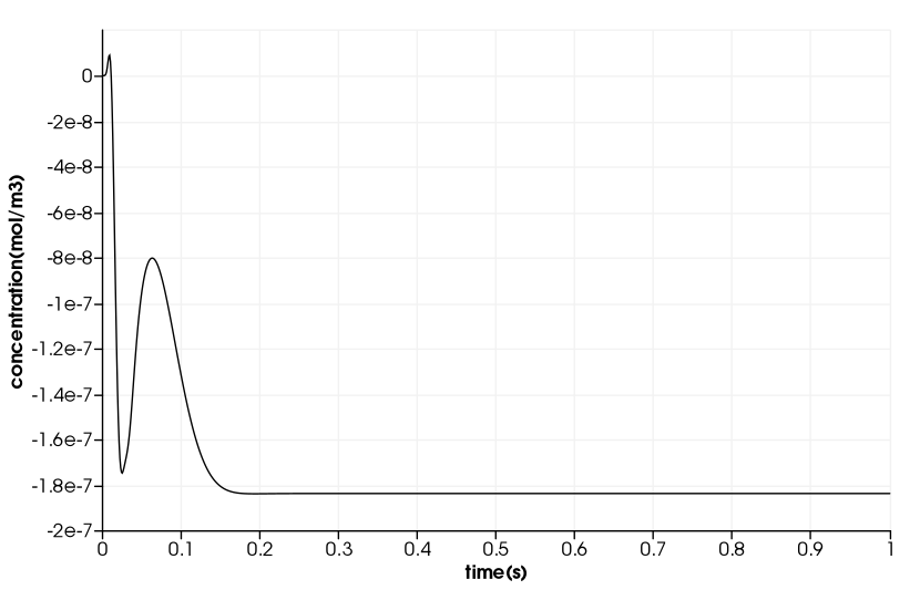
},3.1.6. Post Process
"PostProcess": (1)
    {
	     "Exports":  (2)
	      {
          "fields":["temperature","pid"] (3)
        },
         "Measures": (4)
        {
            "Points": (5)
            {
                "pointA": (6)
                {
                    "coord":"{0,R/2.0, 9e-3}", (7)
                    "fields":"temperature" (8)
                }
            }
        }
}| 1 | the name of the section |
| 2 | the Exports identifies the toolbox fields that have to be exported for visualisation |
| 3 | the list of fields to be exported |
| 4 | the Mesures identifies the toolbox |
| 5 | the type of area to be measured, here Point |
| 6 | the name of the Point, here "pointA" |
| 7 | the coordinates of the point "pointA" |
| 8 | the type of measure to do, here temperature |
3.2. CFG file
The Model CFG (.cfg) files allow to pass command line options to Feel++ applications. In particular, it allows to
-
setup the mesh
-
define the solution strategy and configure the linear/non-linear algebraic solvers.
directory=Stent2DExport/1 (1)
case.dimension=3 (2)
case.discretization=P1 (3)

[heat] (4)
mesh.filename=$cfgdir/arterial3d_v3.msh (5)
#gmsh.hsize=2e-4#0.01#0.05

filename=$cfgdir/arterial2d.json (6)

velocity-convection={0,0,umax*((R^2)-(x^2)_(y^2))/(R^2)}:umax:R:x:y:D (7)
initial-solution.temperature=0 (8)

pc-type=lu #gasm (9)
do_export_all=1 (10)

ksp-maxit=1000 (11)
stabilization-gls=1 (12)

ksp-rtol=1e-20 (13)
snes-rtol=1e-20 (13)
snes-ksp-rtol=1e-20 (13)

[heat.bdf]
order=2 (14)

[ts]
time-step=1e-4 (15)
time-final=1 (16)
#restart.at-last-save=true (17)| 1 | the directory where the results are exported: 1 for part1 and 2 for part2 |
| 2 | the dimension of the application, by default 3D |
| 3 | we use \(\mathbb{P1}\) |
| 4 | toolbox prefix |
| 5 | the mesh file |
| 6 | the associated Json file |
| 7 | the velocity expression |
| 8 | the initial solution: here the temperature take the role of the concentration |
| 9 | the chosen method for decomposition |
| 10 | to export all result |
| 11 | to change the maximum iteration for each step |
| 12 | as we compute convection, we need to apply stabilisation |
| 13 | to change the tolerance into \(1e-20\) |
| 14 | heat.bdf |
| 15 | time step : 1e-4s |
| 16 | time final : 1s |
| 17 | restart at last save |