 .pdf
.pdf
Heat transfer Modeling and Theory
1. What is Heat Transfer?
1.1. Heat transfer modes
Heat transfer is the energy transfer process as a result of temperature difference.
A thermal analysis is undertaken to predict temperatures and heat transfer within and around bodies. This information may then be used to model temperature dependent phenomenon such as thermally induced stresses or the effect on fluid flow in the case of a solidifying metal. Heat flow has been categorised into three different modes.
- Conduction
-
In a solid body, the energy is transferred from a high temperature region to a low temperature region. The rate of heat transfer per unit area is proportional to the temperature gradient in the normal direction. This mode of heat transfer is referred to as conduction.
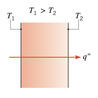 Figure 1. Conduction through a solid or a stationary fluid
 - Convection
-
Convection heat transfer determines the heat flow between a solid body and the surrounding atmosphere of either gases or liquid. In the heat transfer literature, the term 'fluid' generally encompasses both gases and liquid. The convection heat transfer is either forced convection where the fluid is forced to flow around the solid body or natural convection where the fluid flow is due to density variations arising from the heat transfer process.
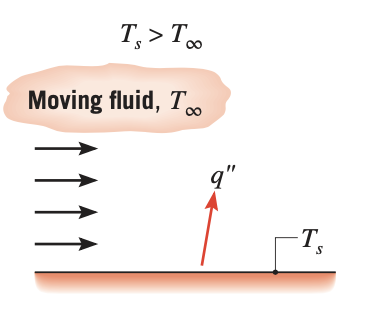 Figure 2. Convection from a surface to a moving fluid
 - Radiation
-
In this mode of heat transfer, the heat flow can occur between a solid body and the surrounding atmosphere with or without the presence of gases or liquid. The heat flows by electromagnetic radiation. This means that heat flow can occur even if the solid body is kept in a vacuum.
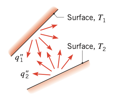 Figure 3. Net radiation heat exchange between two surfaces
The heat conducted through a solid is convected as well as radiated from its surface to the atmosphere. The Figure below illustrates a particular case of this phenomenon. It is assumed that the temperature at the surface 1 is maintained at \(T_{1} K\) and is greater than the ambient temperature \(T_{\infty} K.\) As a result, the heat will conduct through the solid and dissipate into the atmosphere by the means of radiation and/or convection across the boundary surface 2.
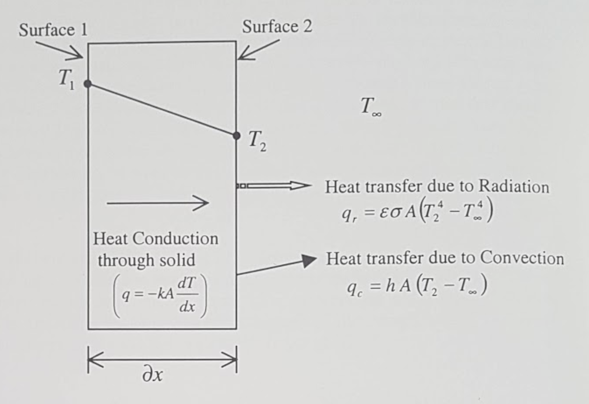
- \(q, q_{c}, q_{r}\)
-
Rate of heat transfer due to conduction, convection and radiation respectively \((W)\)
- \(A\)
-
Cross sectional area normal to heat flow (at surface 1 and } 2 \(\left(m^{2}\right)\)
- \(k, h, \varepsilon, \sigma\)
-
Conductivity \((W / m K),\) convection heat transfer coefficient \(\left(W / m^{2} K\right),\) emissivity and the Stefan Boltzmann constant \(\left(W / m^{2} K^{4}\right)\) respectively.
- \(T_{1}, T_{2}, T_{\infty}\)
-
Temperature at surfaces 1 and \(2,\) and the ambient temperature \((K)\) respectively \(\left(T_{1}>T_{2}>T_{\infty}\right)\)
From the modelling viewpoint, the conduction equation is numerically solved within a solid domain to determine the temperature variation.
Heat transfer due to radiation and convection occur only at the boundary of the solid and are, hence, included as boundary conditions.
The boundary of the solid may also be maintained at a fixed temperature or it may be insulated. Such identification of boundary conditions is necessary in order to solve the conduction equation.
1.2. Why thermal analysis?
There are many reasons for undertaking thermal analyses. In the context of engineering and in its simplest form, thermal analysis may be used to
- Estimate the temperature distribution within a component or assembly
-
This may be important where temperature is a key factor with regard to integrity or where differential thermal expansion causes internal stresses. Contrasting examples include microelectronic components that are subjected to a working load cycle and large structures that are subject to a fire risk.
- Calculate the temperature distribution in a component
-
it may be possible to establish heat flows that are present where energy transfer is a primary consideration (e.g. heat exchanger and condenser).
Thermal calculations are frequently coupled with other types of analysis:
-
fluid flow and
-
structural analysis.
1.2.1. Heat transfert and Structural Snalysis
The coupling of heat transfer and structural analysis comprises a common application: A structure or a material either contracts or expands when subjected to temperature changes.
The thermal contraction or expansion is directly proportional to the temperature changes and is characterised by a coefficient of linear expansion
where \(\Delta \varepsilon\) is the change in strain taking place in the body, \(\alpha\) is the coefficient of thermal expansion and \(\Delta T\) is the temperature change. The value of the coefficient of linear expansion is determined experimentally on very small samples and therefore represents an unrestrained system. However, in a structure, it represents initial strains in the body and can be converted into stresses and forces to be used as the load vector in the finite element structural analysis. In most practical applications, the contraction or expansion of the structure is partially or fully constrained thus inducing internal stresses. This can be important where thermally induced stresses may cause failure, where thermal distortion control is a requirement, or where residual stresses need to be evaluated in the case of components that are cooled (e.g. castings, heat treatment etc.).
1.2.2. Heat transfer and Other Physics
More complex systems also require thermal analysis:
- Chemical reaction
-
it must incorporate a model of thermal generation that arises as a consequence of the reaction.
- Phase change
-
Heat transfer with phase change has also become an important field because a large number of industrial applications (e.g. metal casting, plastics, injection moulding and other forming processes.) address this as part of a manufacturing process simulation. For example, the transient temperatures in a casting (or an injection moulded component) are important since they point to potential areas in the casting that may be defective, or they provide an indication of the duration of the cooling cycle.
1.3. Purpose of Thermal Analysis
Before an analysis is undertaken, it is important to establish the purpose of the investigation, since this motivates the study and defines some of the inputs and the output requirements from the analysis. * if temperature limits are a concern, then the temperature field throughout the system is the important output. * if the analysis goal is to establish cooling, then heat flux is likely to be more important and this will be displayed as an output.
| A good understanding of the underlying physical principles of the thermal analysis is a basic requirement for its correct application in any modelling task, in that the model must be 'fit for purpose'. |
The purpose of the analysis will also influence the input detail for the model. This is a key issue since this actually defines the thermal model. These details include the geometry, which may need to be abstracted from a design drawing or even from a sketch at the design feasibility stage, material properties and thermal boundary conditions. In the case of a transient thermal analysis this also requires the input of an initial temperature field together with time stepping information. This, similar to a structural analysis, the model input comprises abstracted geometry, material properties, constraints and loads.
The thermal analysis is classified into four categories. The classification is based on whether the heat transfer problem is time dependent and material properties or boundary conditions vary with respect to the temperature.
The simple flow diagram summarises the classification process.

Mode |
Mechanism(s) |
Rate Equation |
Transport Property or Coefficient |
Conduction |
Diffusion of energy due to random molecular motion |
\(q_{x}^{\prime \prime}\left(\mathrm{W} / \mathrm{m}^{2}\right)=-k \nabla T\) |
\(k(\mathrm{W} / \mathrm{m} \cdot \mathrm{K})\) |
Convection |
Diffusion of energy due to random molecular motion plus energy transfer due to bulk motion (advection) |
\(q^{\prime \prime}\left(\mathrm{W} / \mathrm{m}^{2}\right)=h\left(T_{s}-T_{\infty}\right)\) |
\(k(\mathrm{W} / \mathrm{m}^2 \cdot \mathrm{K})\) |
Radiation |
Energy transfer by electromagnetic waves |
\(\begin{aligned} q^{\prime \prime}\left(\mathrm{W} / \mathrm{m}^{2}\right) &=\varepsilon \sigma\left(T_{s}^{4}-T_{\mathrm{sur}}^{4}\right) \\ \text { or } q(\mathrm{W}) &=h_{r} A\left(T_{s}-T_{\mathrm{sur}}\right) \end{aligned}\) |
\(\begin{aligned}\varepsilon\\ h_{r}\left(\mathrm{W} / \mathrm{m}^{2} \cdot \mathrm{K}\right)\end{aligned}\) |
2. Nomenclature and Units
| Notation | Quantity | Unit |
|---|---|---|
\(A\) |
Area |
\(m^{2}=10^{6} \mathrm{mm}^{2}=10^{4} \mathrm{cm}^{2}\) |
\(\rho\) |
Density |
\(k g / m^{3}=10^{3} g / c m^{3}\) |
\(t\) |
Time |
\(S\) (second) |
\(T\) |
Temperature |
\(C\) (degree Celsius), \(K\) (degree Kelvin) |
\(C_p\) |
Specific heat |
\(J / k g C=J / k g K\) |
\(k\) |
Conductivity |
\(W / m C=W / m K\) |
\(h\) |
Convection heat transfer coefficient |
\(W / m^{2} C=W / m^{2} K\) |
\(q\) |
Rate of heat transfer |
\(W\) |
\(\sigma\) |
Stefan Boltzmann constant |
\(W / m^{2} K^{4}\) |
\(\mathcal{E}\) |
Emmissivity |
Process |
\(h\) \(\left(\mathrm{W} / \mathrm{m}^{2} \cdot \mathrm{K}\right)\) |
Free convection |
|
Gases |
\(2-25\) |
Liquids |
\(50-1000\) |
Forced convection |
|
Gases |
\(25-250\) |
Liquids |
\(100-20,000\) |
Convection with phase change |
|
Boiling or condensation |
\(2500-100,000\) |
3. Heat Transfer Theory
Assumptions
-
you are familiar with heat transfer and have read the introduction.
-
you have read the notations, units and glossary.
3.1. Equations
which is completed with boundary conditions and initial value
3.1.1. Convective heat transfer
3.1.2. Steady case
3.1.3. Multi-materials
Given a domain \(\Omega \subset \mathbb{R}^d, d=1,2,3\), \(\Omega\) is partitioned into \(N_r\) regions \(\Omega_i,i=1,\ldots,N_r\) corresponding to different materials (solid or fluid). We consider \(\rho_i\), \(C_{p,i}\) and \(k_i\) the material properties defined in each regions \(\Omega_i\). We define also \(\boldsymbol{n}_i\) the outward unit normal vector associated to the boundary \(\partial \Omega_i\).
We assume the operator \(\mathcal{L}\) tel que \(\mathcal{L} T = \rho_i C_{p,i} \frac{\partial T}{\partial t} - \nabla \cdot \left( k_i \nabla T \right)\) is elliptical.
We multiply \(\mathcal{L} u = Q\) by a function test \(v \in \mathbf{V}\) and integrates by part on \(\Omega_i\). Which give:
By the formula of Green, we get
Additivity of the integral, we have
Note that
Use the conditions in the interfaces, we get
Using the implicit Euler method for the time term:
Denoting \(T^k = T(t^k)\), we write the formula in \(t^{ k+1}\), we obtain:
So, the weak wording becomes:
So we have \(a(u_{k+1},v)\) a continuous bilinear form coercive in \(v \in \mathbf{V}\) and \(l(\phi)\) a continuous linear form . We are in a Hilbert space, so we have all the conditions for the application of the Lax-Milgram theorem. So this problem is well posed.
Correct approximation:
We use the Galerkin approximation method:
Let \(\{ \mathcal{T}_h \}\) a family of meshes of \(:\Omega\).
Let \(\{ \mathcal{K}, P, \sum \}\) a finite element of Lagrange of reference of the degree \(k \geq 1\).
Let \(P^k_{c,h}\) the conforming approximation space defined by
To obtain a conformal approximation in V, we add the boundary conditions
Discrete problem is written:
Let \(\{ \varphi_1, \varphi_2, ..., \varphi_N \}\) the base of \(V_h\). An element \(T_h \in V_h\) is written as
Using \(v\) as a basic function of \(V_h\), our problem becomes
The variational problem of approximation is then equivalent to a linear system
Introduce
We write the system in matrix form
3.1.4. Variational formulation and discretization of the heat equation with radiative boundary conditions on several surfaces
| Radiative heat transfer is not yet available in the toolboxes. An application implementing radiative heat is currently available in feelpp/doc/manual/heat. |
Let \(\partial\Omega_D\) and \(\partial \Omega_N\) be the portions of the boundary where Dirichlet and Neumann boundary conditions are applied, respectively. Let us write the variational formulation of the heat equation: find \(T \in H^1((0,T);H^1(\Omega))\) such that, for all \(\phi \in H^1_{0,\partial \Omega_D}(\Omega)\)
When the radiative boundary \(\partial \Omega_R\) is composed of several subsurfaces that can exchange heat through radiation, the associated radiative boundary condition is complex. In fact, each surface receives heat contributions from the other ones, proportionally to the values of the corresponding view factors. From Modest’s book [Radiative_heat_transfer], equation (5.28), the radiative heat flux at point \(x\) of \(\partial \Omega_R\) is
In this equation, \(q=\nabla T \cdot \vec{n}, E_b(x)=\sigma T^4\), \(\epsilon(x)\) is the emittance and \(dF_{x-x'}\) is the view factor between the infinitesimal areas surrounding points \(x,x'\).
Picard’s iteration
Let us now propose a variational formulation for this equation. Let \(\psi \in \mathbb{P}^0_{d}(\partial \Omega_R)\) be discontinuous, piecewise constant basis functions. Functions \(\psi\) are elementwise discontinuous; however, one could choose to work, as a first approximation, with \(\Psi \in P\), where \(P\) a space of discontinuous, piecewise constant basis functions, where discontinuities are not elementwise, but for example discontinuous in correspondence of different radiating surfaces. In the following, we will use \(\psi\) to denote test functions and \(N_h\) to denote the cardinality of the test space. We have
By decomposing \(q(x)=\sum_{i=0}^{N_h} q_i \psi_i(x)\), the first term of the left-hand side gives rise to a mass matrix \(M_{ij} = \int_{\partial \Omega_R} \epsilon_i^{-1} \psi_i\psi_j\). The non-linearity in \(q\) is handled iteratively: the second term on the left-hand side is treated explicitly and moved to the right-hand side. It can be decomposed as a function of coefficients \(q_i\) as \(N_{j}(q) = \int_{\partial \Omega_R} \Big( \sum_{A_k} \frac{1}{A_k} \int_{A_k} (\frac{1}{\epsilon_k}-1) q_k F_{ik} \, dA \Big)\psi_j\). The right-hand side is of the form \(D_j(T) = \int_{\partial \Omega_R} ( \sigma T^4 + \sum_{A_k} \frac{1}{A_k} \int_{A_k} T^4_k F_{jk} \, dA) \psi_j\).
Due to the presence of the fourth power of the temperature and the non-linearity of the equation with respect to temperature and heat flux, two nested iterative loops are proposed. In the following algorithm, \(n\) denotes time indices, \(k\) denotes the indices of the temperature loop and \(l\) denotes the indices of the flux loop.
\begin{algorithm}
    \caption{Solution of the heat equation with radiative BC on the timestep $\Delta t$.}
    \begin{algorithmic}
    \STATE $T^{n}=T^{n,0}$, $q^{n}=q^{n,0,0}$
    \STATE $T^{n+1,0} = Heat_{\Delta t}(T^n,q^{n})$;
    \STATE $q^{n+1,0,0} = q^{n}$
    \WHILE{$||T^{n+1,k+1} -T^{n+1,k}||/||T^{n+1,0}|| > \tau_T$}
        \STATE $T^{n+1,k} \leftarrow T^{n+1,k+1}$
        \STATE $q^{n+1,k,0} = M_{ij}^{-1} (D_j(T^{n+1,k})-N_{ij}(q^{n+1,k+1,0}))$
        \WHILE{$||q^{n+1,k,l} -q^{n+1,k,l-1}||/||q^{n+1,k,0}|| > \tau_q$}
            \STATE $q^{n+1,k,l-1} \leftarrow q^{n+1,k,l}$
            \STATE $q^{n+1,k,l} = M_{ij}^{-1} (D_j(T^{n+1,k})-N_{j}(q^{n+1,k,l-1}))$
        \ENDWHILE
        \STATE $q^{n+1,k+1,0} \leftarrow q^{n+1,k,l}$
        \STATE $T^{n+1,k+1} = Heat_{\Delta t}(T^{n+1,k},q^{n+1,k+1,0})$
    \ENDWHILE
    \STATE $T^{n+1} \leftarrow T^{n+1,k+1}$
    \STATE $q^{n+1} \leftarrow q^{n+1,k+1,0}$
    \end{algorithmic}
\end{algorithm}
Newton non-linear iteration
The previous integral equation can be included in the variational formulation of the PDE as a boundary condition on the heat flux \(q(x)=\Big(-k \nabla T \cdot n \Big)(x)\):
The linearization of the boundary condition generates the following terms to be added to the Jacobian matrix \(DF(T)\), at iteration \(k\),
The following term is added to the residual \(F(T)\) at iteration \(k\), where we denoted by \(A\) and \(A'\) the areas surrounding points \(x\) and \(x'\).
In practice, the surface of the cavity is divided into smaller surfaces and the view factors \(F_{ij}\) are often already computed and stored for all pairs \(ij\) of (finite) subsurfaces. In that case, the differential \(dF_{dA-dA'}\) can be substituted by the ratio \(F_{ji}/|A_i|\). The meaning of \(dF_{dA-dA'}\) is ``the ratio (diffuse energy leaving $dA$ and intercepted by \(dA'\))/(total energy leaving \(dA\)) '', and the ratio \(F_{ji}/|A_i|\) corresponds to the ratio of (energy leaving surface $j$ and intercepted by surface \(i\))/(total energy leaving surface \(j\)) divided by the area of the intercepting surface. The idea behind the substitution is that integrals \( \Big(\int_{A'} \sigma T^4_k(x') dF_{dA-dA'}\Big) \) and \(\Big(\int_{A'} \Big( \frac{1}{\epsilon(x')} -1\Big)(-k\nabla T_k \cdot \vec{n}) dF_{dA-dA'} \Big)\) produce values for all \(x\in A\), by attributing them a portion of incident radiation which is proportional to the view factor. By dividing \(F_{ji}\) by \(|A_i|\) we construct a density for the view factor, constant over the whole receiving surface, to average the incoming radiation. We hence make the approximation that \( dF_{dA-dA'} = \cos(\theta_i)\cos(\theta_j)/(\pi S^2)dA' \approx F_{ji}/|A_i| dA' = F_{ij}/|A_j| dA' \).
3.2. Bibliography
[Radiative_heat_transfer] Modest, M.F., Radiative Heat Transfer, Elsevier Science (2013) doi.org/10.1016/C2010-0-65874-3
Glossary
- Conductivity
-
Conductivity of a solid is the heat flow per unit area in the normal direction within the solid body as a result of temperature difference.
- Heat flux(conduction)
-
The heat flux by conduction \(q''(W/m2)\) is the heat transfer rate per unit area perpendicular to the direction of transfer, and it is proportional to the temperature gradient in this direction. We have the Fourier law in the multi-dimensional case:
\[q'' = -k \nabla T\] - Heat Rate(conduction)
-
The heat rate by conduction, \(q (W)\), through a plane wall of area \(A\) is then the product of the flux and the area, \(q = q'' \cdot A\).
- Specific heat
-
It is the energy required to raise the temperature of unit mass through one degree temperature rise.
- Adiabatic condition
-
An adiabatic condition means that heat is not allowed to transfer across the boundary. In other words it means a perfectly insulated boundary. Symmetry boundaries are adiabatic.
- Emmissivity
-
This terminology is used in the context of radiation. It is the ratio of the total energy emitted by a surface to the total energy emitted by a black surface at the same temperature.
- View factor
-
In the radiation heat transfer context, it is the ratio of the energy incident on the second body to the energy emitted by the first body. Sometimes, it is also referred to as a geometric factor or form factor.
- Thermal stress
-
Stress induced in a structure or body as a result of thermal loading.
- Phase change
-
Substance subjected to temperature changes may transfer from solid state to liquid and/or gaseous state. During change of phase the latent heat is either released or absorbed.