Linear Compliant Elliptic Problems
- 1. Notations, Definitions, Problem Statement, Example
- 2. Reduced Basis Approximation
1. Notations, Definitions, Problem Statement, Example
1.1. Inner Product Spaces
1.1.1. Definitions
A space \(Z\) is a linear or vector space if, for any \(\alpha \in \mathbb{R}\) , \(w,v \in Z\), \(\alpha w+v \in Z\)
| \(\mathbb{R}\) denotes the real numbers, and \(\mathbb{N}\) and \(\mathbb{C}\) shall denote the natural and complex numbers, respectively. |
An inner product space (or Hilbert space) \(Z\) is a linear space equipped with
-
an inner product \((w,v)_Z, \forall w,v \in Z\), and
-
induced norm \(\|w\|_Z = (w,w)_Z, \forall w \in Z\).
Inner Product : An inner product \(w,v \in Z \rightarrow (w,v)_Z \in \mathbb{R}\) has to satisfy
-
Bilinearity :
-
\((\alpha w+v,z)_Z =\alpha(w,z)_Z +(v,z)_Z \forall \alpha\in R,w,v,z\in Z\)
-
\((z,\alpha w+v)_Z =\alpha(z,w)_Z +(z,v)_Z, \forall \alpha\in R, w,v,z\in Z \)
-
-
Symmetry : \((w,v)_Z = (v,w)_Z, \forall w,v \in Z\)
-
Positivity :
-
\((w,w)_Z >0, \forall w \in Z, w \neq 0\)
-
\((w,w)_Z =0\) only if \(w=0\)
-
Cauchy-Schwarz inequality: \((w,v)_Z \leq \|w\|_Z\|v\|_Z,\forall w, v \in Z\)
1.1.2. Norm
A norm is a map \(\| \cdot \| : Z \rightarrow \mathbb{R}\) such that
-
\(\|w\|_Z > 0\quad \forall w\in Z,w\neq 0,\)
-
\(\|\alpha w\|_Z = |\alpha |\|w\|_Z\quad \forall \alpha \in \mathbb{R},\ \forall w\in Z, \)
-
\(\|w+v\|_Z \leq \|w\|_Z +\|v\|_Z\quad \forall w\in Z,\ \forall v\in Z.\)
Equivalence of norms \(\| \cdot \|_Z\) and \(\| \cdot \|_Y\) : there exist positive constants \(C_1\), \(C_2\) such that \(C_1\|v\|_Z \leq \|v\|_Y \leq C_2\|v\|_Z\).
1.1.3. Cartesian Product Space
Given two inner product spaces \(Z_1\) and \(Z_2\), we define \(Z = Z_1 \times Z_2 \equiv \{(w_1,w_2)\ | \ w_1 \in Z_1,\ w_2 \in Z_2\}\) and given \(w = (w_1,w_2) \in Z, v = (v_1,v_2) \in Z\), we define \(w + v \equiv (w_1 + v_1, w_2 + v_2).\).
We also equip \(Z\) with the inner product \((w,v)_Z =(w_1,v_1)_{Z_1} +(w_2,v_2)_{Z_2}\) and induced norm \(\|w\|_Z = (w,w)_Z\).
1.2. Linear and Bilinear Forms
1.2.1. Linear Forms
A functional \(g : Z \rightarrow \mathbb{R}\) is a linear functional if, for any \(\alpha \in \mathbb{R}, w, v \in Z\) \(g(\alpha w + v) = \alpha g(w) + g(v)\)
A linear form is bounded, or continuous, over \(Z\) if \(|g(v)| \leq C \|v\|_Z, \forall v \in Z,\) for some finite real constant \(C\).
1.2.2. Dual Spaces
Given \(Z\), we define the dual space \(Z'\) as the space of all bounded linear functionals over \(Z\). We associate to \(Z'\) the dual norm \(\|g\|_{Z'} = \displaystyle\sup_{v \in Z} \frac{g(v)}{\|v\|_Z} , \forall g \in Z'\).
For any \(g \in Z'\), there exists a unique \(w_g \in Z\) such that \((w_g, v)_Z =g(v), \forall v \in Z\).
It directly follows that \(\|g\|_{Z'} = \|w_g\|_Z\)
1.2.3. Bilinear Forms
A form \(b:Z_1 \times Z_2 \rightarrow \mathbb{R} \) is bilinear if, for any \(\alpha \in R\),
-
\(b(\alpha w + v,z) = \alpha b(w,z) + b(v,z), \forall w,v \in Z_1, z \in Z_2 \)
-
\(b(z,\alpha w + v) =\alpha b(z,w) + b(z,v), \forall z \in Z_1, w,v \in Z_2\)
The bilinear form \(b : Z \times Z \rightarrow \mathbb{R}\) is
-
symmetric, if \(b(w,v) = b(v,w),\)
-
skew-symmetric, if \(b(w,v) = -b(v,w),\)
-
positive definite, if \(b(v,v) \geq 0\text{ , with equality only for } v = 0.\)
-
positive semidefinite, if \(b(v,v) \geq 0, \forall v \in Z.\)
We also define, for a general bilinear form \(b : Z \times Z \rightarrow \mathbb{R}\), the
-
symmetric part as \(b_S(w,v) = 1/2 (b(w,v) + b(v,w)), \forall w,v \in Z;\)
-
the skew-symmetric part as \(b_{SS}(w,v) = 1/2 (b(w,v) - b(v,w)), \forall w,v \in Z.\)
The bilinear form \(b : Z \times Z \rightarrow \mathbb{R}\) is
-
coercive over \(Z\) if \(\alpha \equiv \inf_{w\in Z} \frac{b(w,w)}{\|w\|^2_Z}\) is positive;
-
continuous over \(Z\) if \(\gamma \equiv \sup_{w\in Z} \sup_{v\in Z} \frac{b(w, v)}{\|w\|_Z \|v\|_Z}\) is finite.
1.2.4. Parametric Linear and Bilinear Forms
We introduce
-
\(D \subset \mathbb{R}^P\) : closed bounded parameter domain;
-
\(\mu = (\mu_1,\ldots,\mu_P) \in D\) : parameter vector.
We shall say that
-
\(g:Z\times D\rightarrow \mathbb{R}\) is a parametric linear form if, for all \(\mu \in D, g( \cdot ; \mu) : Z \rightarrow \mathbb{R}\) is a linear form;
-
\(b:Z\times Z\times D\rightarrow \mathbb{R}\) is a parametric bilinear form if,for all \(\mu \in D, b( \cdot , \cdot ; \mu) : Z \times Z \rightarrow \mathbb{R}\) is a bilinear form.
Concepts of symmetry directly extend to the parametric case.
1.2.5. Parametric Linear and Bilinear Forms
The parametric bilinear form \(b : Z \times Z \times D \rightarrow \mathbb{R}\) is
-
coercive over Z if \(\alpha(\mu) \equiv \inf_{w \in Z} \frac{b(w,w;\mu)}{\|w\|^2_Z}\) is positive for all \(\mu \in D\);
-
continuous over \(Z\) if \(\gamma(\mu)\equiv \sup_{w \in Z} \sup_{v \in Z} \frac{b(w, v; \mu)}{\|w\|_Z\|v\|_Z}\) is finite for all \(\mu \in D.\)
We also define
1.2.6. Coercivity EigenProblem
We have \(\alpha (\mu) \equiv \inf_{w \in Z} \frac{b_S(w,w;\mu)}{\|w\|^2_Z}\)
THe associated generalized eigenproblem is :
Given \(\mu \in D\), find \((\chi^{co},\nu^{co})_i(\mu) \in Z \times \mathbb{R}, 1 \leq i \leq \dim(Z),\) such that \(b_S(\chi_i^{co}(\mu), v; \mu) = \nu_i^{co}(\mu)(\chi_i^{co}(\mu), v)_Z\) and \(\|\chi_i^{co}(\mu)\|_Z=1\).
Let \(\nu_1^{co}(\mu) \leq \nu_2^{co}(\mu) \leq \ldots \leq \nu_{\dim{Z}}^{co} (\mu)\) and \(b\) coercive, then \(\alpha (\mu) = \nu_1^{co}(\mu) > 0.\)
1.2.7. Parameter affine Dependence
We assume \(g(v;\mu)= \displaystyle\sum_{q=1}^{Q_g} \theta^q_g(\mu)g^q(v), \forall v \in Z,\) where, for \(1 \leq q \leq Q_g\) (finite),
-
parameter-dependant functions \(\theta^q_g : D \rightarrow \mathbb{R}\),
-
parameter-independant forms \(g^q : Z \rightarrow \mathbb{R};\)
and \(b(w,v;\mu)= \displaystyle\sum_{q=1}^{Q_b} \theta^q_b(\mu) b^q(w,v),\quad \forall w,v \in Z,\) where, for \(1 \leq q \leq Q_b\) (finite),
-
parameter-dependant functions \(\theta^q_b : D \rightarrow \mathbb{R}\),
-
parameter-independant forms \(b^q : Z \times Z \rightarrow \mathbb{R}\).
1.2.8. Parametric Coercivity
The coercive bilinear form \(b : Z \times Z \times D \rightarrow \mathbb{R}\) \(b(w,v;\mu)= \displaystyle\sum_{q=1}^{Q_b} \theta^q_b(\mu) b^q(w,v),\quad \forall w,v \in Z,\) is parametrically corecive if \(c\equiv b_S\) is affine \(c(w,v;\mu)= \displaystyle\sum_{q=1}^{Q_c} \theta^q_c(\mu) c^q(w,v),\quad \forall w,v \in Z,\) and satisfies and
-
\(\theta^q_c(\mu)>0, \forall \mu \in D, 1\leq q\leq Q_c,\)
-
\(c^q(v,v)\geq 0,\forall v \in Z, 1\leq q\leq Q_c.\)
1.3. Classes of Functions
1.3.1. Scalar and Vector Fields
We consider (real)
-
scalar-valued field variables (e.g., temperature, pressure) \(w : \Omega \rightarrow \mathbb{R}^{d=1}\)
-
vector-valued field variables (e.g., displacement, velocity) \(\mathbf{w} : \Omega \rightarrow \mathbb{R}^d\) , where \(\mathbf{w}(x) = (w_1(x), \ldots , w_d (x));\)
and
-
\(\Omega \in \mathbb{R}^d, d=1, 2, \text{or } 3\) is an open bounded domain
-
\(x = (x_1,...,x_d) \in \Omega \);
-
\(\Omega\) has Lipschitz continuous boundary \(\partial \Omega\)
And we define the canonical basis vectors as \(e_i, 1 \leq i \leq d.\)
1.3.2. Multi-Index Derivative
Given a scalar (or one component of a vector)
-
field \(w : \Omega \rightarrow \mathbb{R}\) (SPATIAL DERIVATIVE)
-
parametric field \(w : \Omega \times D \rightarrow \mathbb{R}\) (SENSITIVITY DERIVATIVE)
where
-
\(\sigma = (\sigma_1,\ldots,\sigma_d)\), \(\sigma_i, 1 \leq i \leq d\), non-negative integers;
-
\(|\sigma| = \sum_{j=1}^{d} \sigma_j\) is the order of the derivative; and
-
\(I^{d,n}\) is set of all index vectors \(\sigma \in N^d_0\) such that \(|\sigma | \leq n.\)
1.3.3. Function Spaces
Let \(m \in N_0\), the space \(C^m(\Omega )\) is defined as \(C^m(\Omega )\equiv \{w | D^\sigma w \in C^0(\Omega ), \forall \sigma \in I^{d,m}\},\) and \(C^0(\Omega )\) is the space of continuous functions over \(\Omega \in \mathbb{R}^d\).
We denote by \(C^\infty (\Omega )\) the space of functions \(w\) for which \(D^\sigma\) exists and is continuous for any order \(|\sigma |.\)
1.3.4. Lebesgue Spaces
We define, for \(1 \leq p < \infty\), the Lebesgue space \(L^p(\Omega )\) as \(L^p(\Omega )\equiv \{ w \text{ measurable } | \|w\|_{L^p(\Omega )} < \infty\}\) where
-
\(\|w\|_{L^p(\Omega )} \equiv \left( \int_\Omega |w|^pdx\right)^{1/p} , 1\leq p<\infty,\)
-
\(\|w\|_{L^\infty (\Omega )} \equiv \mathrm{ess} \sup_{x\in\Omega} |w(x)|, p = \infty .\)
1.3.5. Hilbert Space
Let \(m \in \mathbb{N}_0\), the space \(H^m(\Omega )\) is then defined as \(H^m(\Omega )\equiv \{w | D^\sigma w \in L^2(\Omega ), \forall \sigma \in I^{d,m}\},\) with associated inner product \((w,v)_{H^m(\Omega )}\equiv \displaystyle\sum_{\sigma \in I^{d,m}}\int_\Omega D^\sigma w D^\sigma v dx,\) and induced norm \(\|w\|_{H^m(\Omega )} \equiv \sqrt{(w, w)_{H^m(\Omega )}}.\)
1.3.6. Special (most important) cases
Since we only consider second-order PDEs, we require mostly
-
\(L^2(\Omega ) = H^0(\Omega )\): Lebesgue Space \(p = 2\)
-
\((w,v)_{L^2(\Omega)} = \int_\Omega w v \quad \forall w, v \in L^2(\Omega )\)
-
\(\|w\|_{L^2(\Omega)} = \sqrt{(w,w)_{L^2(\Omega)}} \forall w \in L^2(\Omega ),\)
-
\(\Rightarrow\) Space of all functions \(w : \Omega \rightarrow \mathbb{R}\) square-integrable over \(\Omega\) .
-
\(H^1(\Omega)\) \(H^1(\Omega ) \equiv \{w \in L^2(\Omega )| \frac{\partial w}{ \partial xi} \in L^2(\Omega ), 1\leq i\leq d\}\) with inner product and induced norm \((w,v)_{H^1(\Omega )} \equiv \int_\Omega \nabla w \cdot \nabla v + wv\quad \forall w,v \in H^1(\Omega ),\), \(\|w\|_{H^1(\Omega )} \equiv \sqrt{(w,w)_{H^1(\Omega)}}\quad \forall w \in H^1(\Omega ),\) and seminorm \(|w|_{H^1(\Omega )} \equiv \int_\Omega \nabla w \cdot \nabla w,\quad \forall w \in H^1(\Omega ).\)
-
the space \(H_0^1(\Omega )\) \(H^1_0(\Omega) \equiv \{v \in H^1(\Omega )|v_{|\partial \Omega}=0 \}\) where \(v = 0\) on the boundary \(\partial \Omega .\)
Note that, for any \(v \in H_0^1(\Omega )\), we have \(C_{PF} \|v\|_{H^1(\Omega )} \leq |v|_{H^1(\Omega )} \leq \|v\|_{H^1(\Omega )},\) and thus \(\|v\|_{H^1(\Omega)} = 0 \, \Rightarrow v = 0\) \(\Rightarrow |v|_{H^1(\Omega )}\) constitutes a norm for \(v \in H_0^1(\Omega ).\)
1.3.7. Projection
Given Hilbert Spaces \(Y\) and \(Z \subset Y\) , the projection, \(\Pi : Y \rightarrow Z\), of \(y \in Y\) onto \(Z\) is defined as
Properties:
-
Orthogonality: \((y - \Pi y, v)_Y = 0\)
-
Idempotence: \(\Pi (\Pi y) = \Pi y\)
-
Best Approximation \(\|y-\Pi y\|^2_Y = \inf_{v \in Z} \|y-v\|^2_Y, \, \)
Given an orthonormal basis \(\{ \varphi_i\}_{i=1, N = \dim(Z)}\), then \(\Pi y= \sum_{i=1}^{\dim(Z)} ( \varphi_i,y)_Y \varphi_i, \forall y \in Y\)
1.4. Notations
1.4.1. Notations
-
\((\cdot)^\mathcal{N}\) finite element approximation
-
\((\cdot)_N\) reduced basis approximation
-
\(\mu\) input parameter (physical, geometrical,…)
-
\(s(t;\mu) \approx s^\mathcal{N}(t;\mu)\approx s_N(t;\mu) \) output approximations
-
\(\mu \rightarrow s(t;\mu)\) input-output relationship
1.4.2. Definitions
-
\(\Omega \subset \mathbb{R}^d\) spatial domain
-
\(\mu\) \(P\)-uplet
-
\(\mathcal{D}^\mu \subset \mathbb{R}^P \) parameter space
-
\(s\) output, \(\ell, f\) functionals
-
\(u\) field variable
-
\(X\) function space \(H^1_0(\Omega)^\nu \subset X \subset H^1(\Omega)^\nu\) (\(\nu=1\) for simplicity)
\((\cdot,\cdot)_X\) scalar product and \(\|\cdot\|_X\) norm associated to \(X\)
1.5. Problem Statement
The formal problem statement reads: Given \(\mu \in \mathcal{D}^\mu\), evaluate \(s(\mu) = \ell(u(\mu);\mu)\) where \(u(x;\mu) \in X\) satisfies \(a(u(\mu), v; \mu ) = f(v; \mu), \quad \forall v \in X\)
We consider first the case of linear affine compliant elliptic problem and then complexify.
1.5.1. Hypothesis: Reference Geometry
In these notes \(\Omega\) is considered
-
To apply the reduced basis methodology exposed later, we need to setup a reference spatial domain \(\Omega_{\mathrm{ref}}\)
-
We introduce an affine mapping \(\mathcal{T}(\cdot;\mu) : \Omega (\equiv \Omega_{\mathrm{ref}} = \Omega_o(\bar{\mu})) \rightarrow \Omega_o(\mu)\) such that \(a(u,v;\mu) = a_o(u_o \circ \mathcal{T}_\mu,v_o \circ \mathcal{T}_\mu;\mu)\)
1.5.2. Hypothesis: Continuity, stability, compliance
We consider the following \(\mu-\)PDE
\(a(\cdot,\cdot;\mu)\) is :
-
bilinear
-
symmetric
-
continuous
-
coercive (\(\forall \mu \in \mathcal{D}^\mu\))
\(f(\cdot;\mu), \ell(\cdot;\mu)\) are :
-
linear
-
bounded (\(\forall \mu \in \mathcal{D}^\mu\))
and in particular, to start, the compliant case
-
\(a\) symmetric
-
\(f(\cdot;\mu) = \ell(\cdot;\mu)\quad \forall \mu \in \mathcal{D}^\mu\)
1.5.3. Hypothesis: Affine dependence in the parameter
We require for the RB methodology \(a(u,v;\mu) = \displaystyle\sum_{q=1}^{Q_a} \Theta^q_a(\mu)\ a^q( u, v )\) where for \(q=1,...,Q_a\)
Remark :
-
similar decomposition is required for \(\ell(v;\mu)\) and \(f(v;\mu)\), and denote \(Q_\ell\) and \(Q_f\) the corresponding number of terms
-
applicable to a large class of problems including geometric variations
-
can be relaxed (see non affine/non linear problems)
1.5.4. Inner Products and Norms
-
energy inner product and associated norm (parameter dependant) \(\begin{aligned} (((w,v)))_\mu &= a(w,v;\mu) &\ \forall u,v \in X\\ |||v|||_\mu &= \sqrt{a(v,v;\mu)} &\ \forall v \in X \end{aligned}\)
-
\(X\)-inner product and associated norm (parameter independant) \(\begin{aligned} (w,v)_X &= (((w,v)))_{\bar{\mu}} \ (\equiv a(w,v;\bar{\mu})) &\ \forall u,v \in X\\ ||v||_X &= |||v|||_{\bar{\mu}} \ (\equiv \sqrt{a(v,v;\bar{\mu})}) & \ \forall v \in X \end{aligned}\)
1.5.5. Coercivity and Continuity Constants
We assume \(a\) coercive and continuous
Recall that
-
coercitivy constant \((0 < ) \alpha(\mu) \equiv \inf_{v\in X}\frac{a(v,v;\mu)}{||v||^2_X}\)
-
continuity constant \(\gamma(\mu) \equiv \sup_{w\in X} \sup_{v\in X}\frac{a(w,v;\mu)}{\|w\|_X \|v\|_X} ( < \infty)\)
« Truth » FEM Approximation
Let \(\mu \in \mathcal{D}^{\mu}\), evaluate \(\displaystyle s^{\mathcal{N}} (\mu) = \ell (u^{\mathcal{N}} (\mu))\), where \(u^{\mathcal{N}} (\mu) \in X^{\mathcal{N}}\) satisfies \(a (u^{\mathcal{N}} (\mu), v; \mu ) = f (v), \quad \forall \: v \in X^{\mathcal{N}}\). Here \(X^{\mathcal{N}} \subset X\) is a truth finite element approximation of dimension \(\mathcal{N}\gg 1\) equiped with an inner product \((\cdot,\cdot)_X\) and induced norm \(||\cdot||_X\). Denote also \(X'\) and associated norm \(\ell \in X',\qquad\displaystyle ||\ell||_{X'} \equiv \operatorname{sup}_{v\in X}\frac{\ell(v)}{||v||_X}\).
1.5.6. Purpose
-
Equate \(u(\mu)\) and \(u_{\mathcal{N}}(\mu)\) in the sense that \(||u(\mu)-u_{\mathcal{N}}(\mu)||_X \leq \mathrm{tol}\quad\forall \mu \in \mathcal{D}^\mu\)
-
Build the reduced basis approximation using the FEM approximation
-
Measure the error associated with the reduced basis approximation relative to the FEM approximation
\(\Rightarrow u^{\mathcal{N}} (\mu)\) is a calculable surrogate for \(u(\mu).\) \(\|u(\mu)-u^\mathcal{N}(\mu)\|_{X} \leq \underbrace{\|u(\mu)-u^\mathcal{N}(\mu)\|_{X}}_{\leq \varepsilon^\mathcal{N}} + \underbrace{\|u^\mathcal{N}(\mu)-u^N(\mu)\|_X}_{\varepsilon_{\mathrm{tol,min}}}\)
with \(\varepsilon^\mathcal{N} \ll \varepsilon_{\mathrm{tol,min}}\)
2. Reduced Basis Approximation
2.1. Reduced Basis Objectives
For any given accuracy \(\epsilon\), evaluate
that probably achieves the desired accuracy
for a very low cost \(t_{\text{comp}}\) Efficiency
where \(t_{\text{comp}}\) is the time to perform the input-output relationship \(\mu \mapsto (s_N(\mu),\Delta^s_N(\mu))\).
2.2. Rapid Convergence
Build a rapidly convergent approximation of \(s_N(\mu) \in \mathbb{R}\) and \(u_N(\mu) \in X^N \subset X^{\mathcal{N}} \subset X\) such that for all \(\mu\), we have \(s_N(\mu) \rightarrow s^{\mathcal{N}}(\mu)\) and \(u_N(\mu) \rightarrow u^{\mathcal{N}}(\mu)\) rapidly as \(N = \operatorname{dim}{X_N} \rightarrow \infty (= 10-200)\) (and of \(\mathcal{N}\))
2.3. Reliability and Sharpness
Provide a posteriori error bound \(\Delta_N(\mu)\) and \(\Delta^s_N(\mu)\) :
and
for all \(N = 1 \ldots N_{\text{max}}\) and \(\mu \in \mathcal{D}^\mu\).
2.4. Efficiency
Develop a two stage strategy : Offline/Online
- Offline
-
very expensive pre-processing, we have typically that for a given \(\mu \in \mathcal{D}^\mu\) \(t^{\text{offline}}_{\text{comp}} \gg t^{\mu\rightarrow s^{\mathcal{N}}(\mu)}_{\text{comp}}\)
- Online
-
very rapid convergent certified reduced basis input-output relationship \(t^{\text{online}}_{\text{comp}} \text{ independent of } \mathcal{N}\)
\(\mathcal{N}\) may/should be chosen conservatively.
2.5. Parametric Manifold \(\mathcal{M}^\mathcal{N}\)
We assume
-
the form \(a\) is continuous and coercive (or inf-sup stable),
-
affine-dependence,
-
the \(\theta^q(\mu), 1 \leq q \leq Q\), are smooth (i.e., \(\theta^q \in C^\infty(\mathcal{D})\)
then \(\mathcal{M}^\mathcal{N} = \{ u^\mathcal{N}(\mu),\, \mu \in \mathcal{D}\}\) is a smooth \(P\)-dimensional manifold in \(X^\mathcal{N}\), since \(\| D_\sigma y^\mathcal{N}(\mu) \| \leq C_\sigma \forall \mu \in \mathcal{D}\), for any order \(|\sigma| \in \mathbb{N}_{+0}\)
2.6. Low-Dimension Manifold
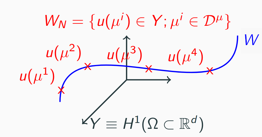
To approximate \(u(\mu)\) and thus \(s(\mu)\), we need not represent all functions in \(Y\). We need only approximate functions in low dimensional manifole \(W = \{ u(\mu)\in Y; \mu\in \mathcal{D}^\mu\}\).
We construct the approximation space \(W_N = \{u(\mu^i)\in Y, (\mu^i)_{i=1...N} \subset \mathcal{D}^\mu\}\)
2.7. Spaces & Bases
We define the RB approximation space \(X_N =\operatorname*{span}\{\xi^n, 1 \leq n \leq N \},\, 1 \leq N \leq N_{max}\) with linearly independent basis functions \(\xi^n \in X,\, 1 \leq n \leq N_{max}\). We thus obtain \(X_N \subset X, \, \operatorname{dim}(X_N) = N,\, 1 \leq N \leq N_{max}\) and \(X_1 \subset X_2 \subset \ldots X_{N_{max}} (\subset X)\).
We denote non-hierarchical RB spaces as \(X^{nh}_N, 1 \leq N \leq Nmax\) \(X^{nh}_N \subset X, \, \operatorname{dim}(X^{nh}_N) = N,\, 1 \leq N \leq N_{max}\)
Parameter Samples : \(S_N = \{ \mu_1 \in \mathcal{D}^{\mu}, \ldots, \mu_N \in \mathcal{D}^{\mu} \}\quad 1 \leq N \leq N_{\mathrm{max}}\), with \(S_1 \subset S_2 \ldots S_{N_\mathrm{max}-1} \subset S_{N_\mathrm{max}} \subset \mathcal{D}^\mu\)
Lagrangian Hierarchical Space : \(W_N = {\rm span} \: \{ \xi^n \equiv \underbrace{ u (\mu^n)}_{u^{\mathcal{N}} (\mu^n)}, n = 1, \ldots, N \}\), with \(W_1 \subset W_2 \ldots \subset W_{N_\mathrm{max}} \subset X^{\mathcal{N}} \subset{X}\)
Sampling strategies?
-
Equidistributed points in \(\mathcal{D}^\mu\)(curse of dimensionality)
-
Log-random distributed points in \(\mathcal{D}^\mu\)
-
See later for more efficient, adaptive strategies
2.7.1. Taylor & Hermite
-
Taylor reduced basis spaces: \(W^{Taylor}_N = \operatorname*{span}\{D_\sigma u(\mu), \forall \sigma \in I^{P,N-1} \}, 1 \leq N \leq N_{max}\), field variable and sensitivity derivatives at one point in \(\mathcal{D}\).
-
Hermite reduced basis spaces: \(W^{Hermite}_N « = » W^{Lagrangian}_N \cup W^{Taylor}_N\) field variable and sensitivity derivatives at several points in \(\mathcal{D}\)
| We will exclusively use Lagrangian RB spaces in this page. |
2.7.2. Orthogonal Basis
Given \(\xi^n = u(\mu^n), 1 \leq n \leq N_\text{max}\) (Lagrange case) we construct the basis set \(\{\zeta^n, 1 \leq n \leq N_\text{max}\}\), from
| \((\zeta^n,\zeta^m)_X = \delta_{nm}, 1 \leq n,m \leq N_\text{max}\) |
Given reduced basis space \(X_N = {\rm span} \: \{ \zeta^n, n = 1, \ldots, N \}, 1 \leq N \leq N_{max}\) we can express any \(w_N \in X_N\) as \(w_N = \displaystyle\sum_{k=1}^N {w_N}_n \zeta^n\) for unique \({w_N}_n \in \mathbb{R}, 1 \leq n \leq N\).
Reduced basis « matrices » \(Z_N \in \mathbb{R}^{\mathcal{N}\times N} , 1 \leq N \leq N_{max}:\) \(Z_N=[\zeta^1,\zeta^2,...,\zeta^N], 1 \leq N \leq N_{max}\) where, from orthogonality, \(Z^T_{N_{max}} X Z^T_{N_{max}} = I_{N_{max}}\), and \(I_M\) is the Identity matrix in \(\mathbb{R}^{M\times M}\).
2.8. Formulation (Linear Compliant Case): a Galerkin method
2.8.1. Galerkin Projection
Given \(\mu \in \mathcal{D}^{\mu}\) evaluate
where \(u_N (\mu) \in X_N\) satisfies
2.8.2. Optimality
For any \(\mu \in \mathcal{D}^\mu\), we have the following optimality results (thanks to Galerkin)
and
and finally \(0 \leq s(\mu)-s_N(\mu) \leq \gamma(\mu)\inf_{v_N \in X_N} ||u(\mu) - v_N(\mu)||^2_X\)
2.8.3. Offline-online decomposition
Expand our RB approximations
Express \(s_N(\mu)\)
where \({u_N}_i(\mu), 1 \leq i \leq N\) satisfies
for \(1 \leq i \leq N\)
2.8.4. Matrix form
Solve \(\underline{A}_N (\mu) \: \underline{u}_N (\mu) = \underline{F}_N\)
where
2.8.5. Complexity analysis
Offline: independent of \(\mu\)
-
Solve: \(N\) FEM system depending on \(\mathcal{N}\)
-
Form and store: \(f^q (\zeta_i)\)
-
Form and store: \(a^q( \zeta_i, \zeta_{j})\)
Online: independent of \(\mathcal{N}\)
-
Given a new \(\mu \in \mathcal{D}^\mu\)
-
Form and solve \(A_N(\mu)\) : \(O(Q N^2)\) and \(O(N^3)\)
-
Compute \(s_N(\mu)\)
Online: \(N << \mathcal{N}\) Online we realize often orders of magnitude computational economies relative to FEM in the context of many \(\mu\)-queries.
2.8.6. Condition number
Proposition : Thanks to the orthonormalization of the basis function, we have that the condition number of \(A_N(\mu)\) is bounded by the ratio \(\dfrac{\gamma(\mu)}{\alpha(\mu)}\).
Proof : * Write the Rayleigh Quotient \(\dfrac{v_N^T A_N(\mu) v_N}{v_N^T v_N}, \quad \forall v_N \in \mathbb{R}^N\) * Express \(v_N = \sum_{n=1}^N v_{N_n} \zeta^n\) * Use coercivity, continuity and orthonormality.