Manipulate Expressions

We start with setting the Feel++ environment and loading the Feel++ library.

Set the Feel++ environment with local repository

import feelpp
import sys
app = feelpp.Environment(["myapp"],config=feelpp.localRepository(""))

python

1. Create and evaluate expressions

An expression is a mathematical expression that can be evaluated at a given point and depend on multiple variables. It can be a scalar, a vectorial or a matricial expression. The expression can be created from a string. The expression can be then evaluated at a given point.

1.1. Scalar expression

Create a scalar expression abd evaluate the expression at a given point (1,2)

expr = feelpp.expr("x+y:x:y") (1)
expr.evaluate({"x":1,"y":2}) (2)

python

1	Create a scalar expression from a string, the symbols are listed at the end of the string using `:` as separator.
2	Evaluate the expression at the point (1,2), it returns a array with one element.

Results

array([3.])

The expression can also be evaluated at a set of points.

Evaluate the expression at a set of points

expr.setParameterValues({"y":2}) (1)
import numpy as np
x=np.linspace(0,1,10) (2)
expr.evaluate("x",x) (3)

python

1	Set the value of the parameter `y` to 2
2	Create a numpy array with 10 points between 0 and 1
3	Evaluate the expression at the 10 equidistributed points between 0 and 1, it returns a array with two elements.

Results

array([2.        , 2.11111111, 2.22222222, 2.33333333, 2.44444444,
       2.55555556, 2.66666667, 2.77777778, 2.88888889, 3.        ])

1.2. Vectorial expression

We start with an expression that depends on two variables x and y and create a vectorial expression with the expression x and y.

Create a vectorial expression abd evaluate the expression at a given point (1,2)

expr21 = feelpp.expr("{x,y}:x:y",row=2,col=1) (1)
expr21.evaluate({"x":1,"y":2}) (2)

python

1	Create a vectorial expression from a string, the symbols are listed at the end of the string using `:` as separator.
2	Evaluate the expression at the point (1,2), it returns a array with two elements.

Results

array([1., 2.])

Now we turn to a vectorial expression with 3 components.

expr31 = feelpp.expr("{x,y,z+x}:x:y:z",row=3,col=1) (1)
expr31.evaluate({"x":1,"y":2,"z":10}) (2)

python

1	Create a vectorial expression from a string, the symbols are listed at the end of the string using `:` as separator.
2	Evaluate the expression at the point (1,2,10), it returns a array with three elements.

Results

array([ 1.,  2., 11.])

1.3. Matricial expression

We start with a 2x2 matricial expression.

Create a matricial expression abd evaluate the expression at a given point (1,2)

expr22 = feelpp.expr("{x+y,x,y,y-x}:x:y", row=2, col=2)  (1)
expr22.evaluate({"x":1,"y":2}) (2)

python

1	Create a matricial expression from a string, the symbols are listed at the end of the string using `:` as separator.
2	Evaluate the expression at the point (1,2), it returns a array with four elements.

Results

array([[3., 1.],
       [2., 1.]])

We now turn to a 3x3 matricial expression.

expr33 = feelpp.expr("{x,y,z,x-y,y-y,z+x+y,z,y,x}:x:y:z",row=3,col=3) (1)
expr33.evaluate({"x":1,"y":2,"z":3}) (2)

python

1	Create a matricial expression from a string, the symbols are listed at the end of the string using `:` as separator.
2	Evaluate the expression at the point (1,2,3), it returns a array with nine elements.

Results

array([[ 1.,  2.,  3.],
       [-1.,  0.,  6.],
       [ 3.,  2.,  1.]])

2. Differentiation

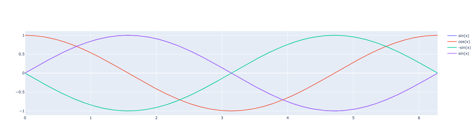
The member functions diff and diff2 allows to compute the first and second symbolic derivatives of a function. The first argument is the symbol with respect to which the derivative is computed.

ex=feelpp.expr("a*sin(x):x:a")
ex.setParameterValues({"a":1})
exd = ex.diff("x") (1)
exd2 = ex.diff2("x") (2)
exda = ex.diff("a") (3)
exdax = ex.diff("a").diff("x") (4)
x=np.linspace(0,2*math.pi,200)
print(f"   ex: {ex}")
print(f"  exd: {exd}")
print(f" exd2: {exd2}")
print(f" exda: {exda}")
print(f"exdaa: {exdax}")

python

1	First derivative with respect to `x` $\frac{\partial \cdot }{\partial x}$
2	Second derivative with respect to `x` $\frac{\partial^2 \cdot }{\partial^2 x}$
3	First derivative with respect to `a` $\frac{\partial \cdot }{\partial a}$
4	First derivative with respect to `a` and then with respect to `x` $\frac{\partial^2 \cdot}{\partial x \partial a}$

Results

   ex: sin(x)*a
  exd: a*cos(x)
 exd2: -sin(x)*a
 exda: sin(x)
exdax: cos(x)

Now let’s plot the expression and its derivative. The first and last are the same.

import plotly.graph_objects as go
fig = go.Figure()
fig.add_trace(go.Scatter(x=x, y=ex.evaluate("x",x), name="sin(x)"))
fig.add_trace(go.Scatter(x=x, y=exd.evaluate("x",x), name="cos(x)"))
fig.add_trace(go.Scatter(x=x, y=exd2.evaluate("x",x), name="-sin(x)"))
fig.add_trace(go.Scatter(x=x, y=exda.evaluate("x",x), name="sin(x)"))
fig.show()

python

Results

2.1. Derivative of a vectorial expression

Here is an example of a vectorial expression and its derivative with respect to x and y.

expr21 = feelpp.expr("{x^3,x*y^2}:x:y", row=2, col=1)  (1)
print("d(x,y)/dx = ",expr21.diff("x")) (2)
print("d(x,y)/dy = ", expr21.diff("y")) (3)
print("d2(x,y)/dxdy = ", expr21.diff("x").diff("y")) (4)
print("d2(x,y)/dydx = ", expr21.diff("y").diff("x"))   (5)

python

1	Create a vectorial expression from a string, the symbols are listed at the end of the string using `:` as separator.
2	First derivative with respect to `x` $\frac{\partial \cdot }{\partial x}$
3	First derivative with respect to `y` $\frac{\partial \cdot }{\partial y}$
4	First derivative with respect to `x` and then with respect to `y` $\frac{\partial^2 \cdot}{\partial x \partial y}$
5	First derivative with respect to `y` and then with respect to `x` $\frac{\partial^2 \cdot}{\partial y \partial x}$

Results

d(x,y)/dx =  [[3*x^2],[y^2]]
d(x,y)/dy =  [[0],[2*x*y]]
d2(x,y)/dxdy =  [[0],[2*y]]
d2(x,y)/dydx =  [[0],[2*y]]

similar results are obtained for matricia expressions.

3. Special functions

The Feel++ library provides a set of special functions that can be used in expressions.

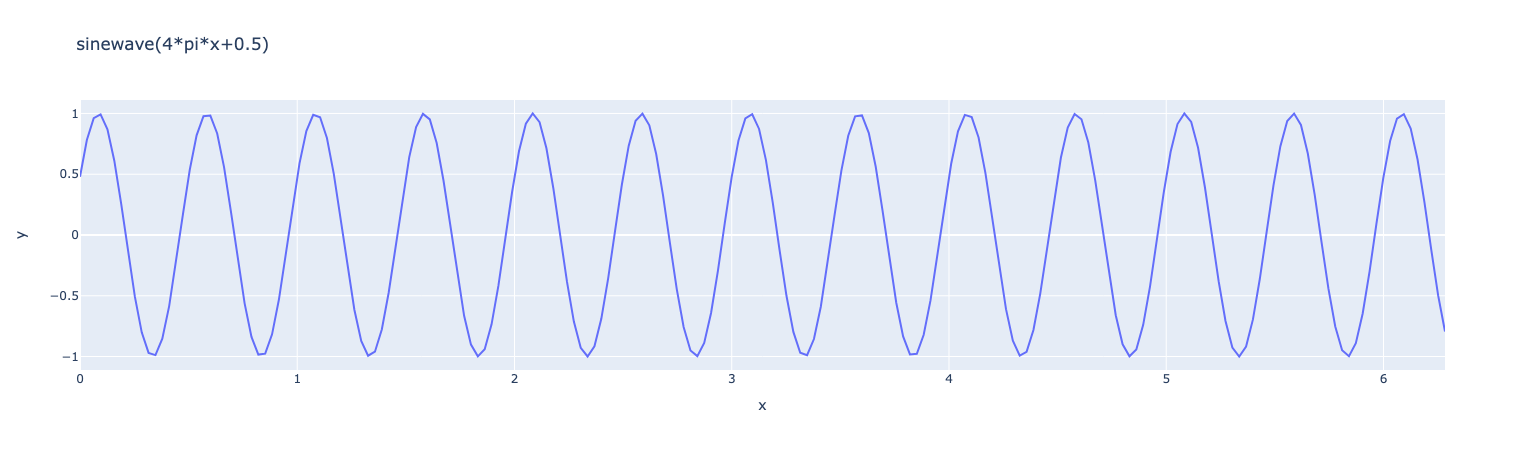
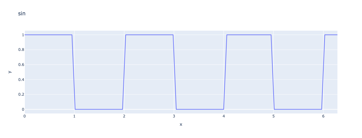
3.1. function with multiple parameters

ex=fpp.expr("sin(w*x+b):x:w:b")
ex.setParameterValues({"w":2*math.pi,"b":0.5})
x=np.linspace(0,2*math.pi,100)
y=ex.evaluate("x",x)

fig = px.line(x=x, y=y, title="sin",labels={"x":"x","y":r'y'})
fig.show()

python

Results

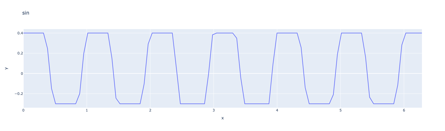
3.2. clamp

The function clamp allows to clamp a value between two bounds.

ex=fpp.expr("clamp(sin(w*x+b),-0.3,0.4):x:w:b")
ex.setParameterValues({"w":2*math.pi,"b":0.5})
x=np.linspace(0,2*math.pi,100)
y=ex.evaluate("x",x)

fig = px.line(x=x, y=y, title="f",labels={"x":"x","y":r'y'})
fig.show()

python

Results

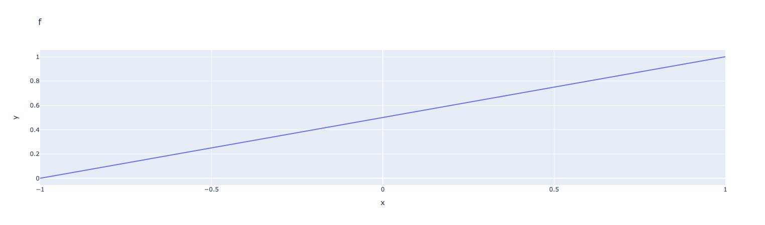
3.3. mapabcd

The function mapabcd allows to map a value from a given interval to another interval. The first argument is the value to map, the second and third arguments are the lower and upper bounds of the interval to map from, the fourth and fifth arguments are the lower and upper bounds of the interval to map to.

ex=fpp.expr("mapabcd(x,-1,1,0,1):x")
x=np.linspace(-1,1,100)
y=ex.evaluate("x",x)

fig = px.line(x=x, y=y, title="f",labels={"x":"x","y":r'y'})
fig.show()

python

Results

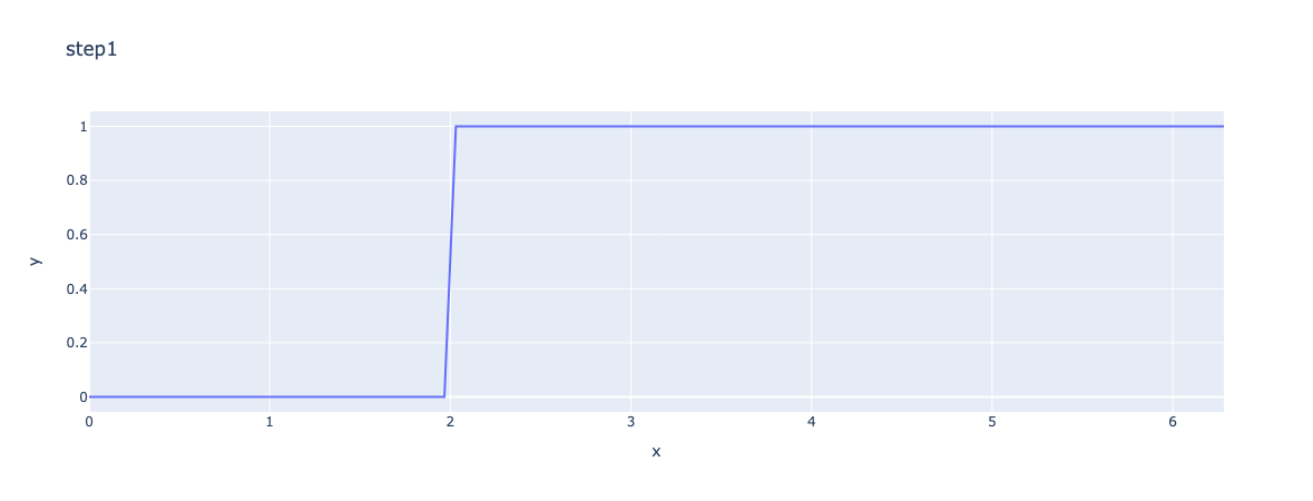
3.4. step1

The function step1 is a step function that is equal to 1 if the argument is greater than 0 and 0 otherwise.

ex=fpp.expr("step1(x,2):x")
x=np.linspace(0,2*math.pi,100)
y=ex.evaluate("x",x)

fig = px.line(x=x, y=y, title="step1",labels={"x":"x","y":r'y'})
fig.show()

python

Results

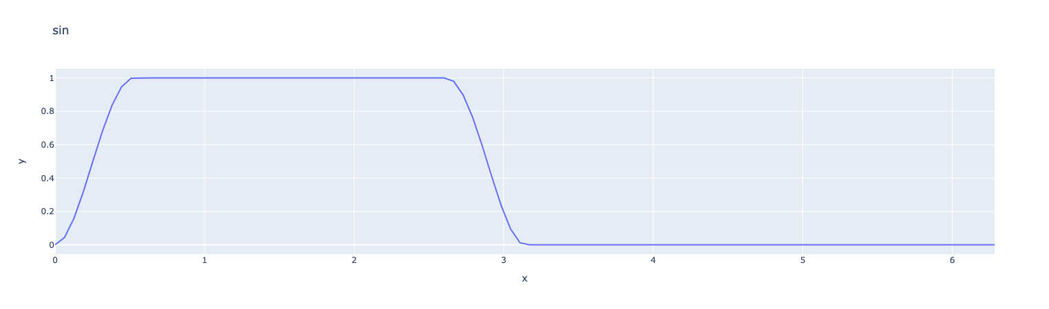
3.5. smoothstep

The smoothstep function is a smooth approximation of the step function.

ex=fpp.expr("smoothstep(sin(x),0,0.5):x")
x=np.linspace(0,2*math.pi,100)
y=ex.evaluate("x",x)

fig = px.line(x=x, y=y, title="smoothstep",labels={"x":"x","y":r'y'})
fig.show()

python

Results

3.6. pulse

The pulse function is defined as $\text{pulse}(x)=\begin{cases} 1 & \text{if } x\in[0,1] \\ 0 & \text{otherwise} \end{cases}$

ex=fpp.expr("pulse(x,0,1,2):x")
x=np.linspace(0,2*math.pi,100)
y=ex.evaluate("x",x)

fig = px.line(x=x, y=y, title="rectangle pulse(0,1,2)",labels={"x":"x","y":r'y'})
fig.show()

python

Results

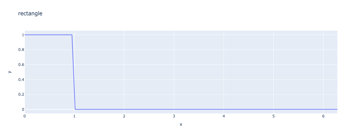
3.7. rectangle

The rectangle function is defined as $\text{rectangle}(x)=\begin{cases} 1 & \text{if } x\in[0,1] \\ 0 & \text{otherwise} \end{cases}$

ex=fpp.expr("rectangle(x,0,1):x")
x=np.linspace(0,2*math.pi,100)
y=ex.evaluate("x",x)

fig = px.line(x=x, y=y, title="rectangle rectangle(0,1)",labels={"x":"x","y":r'y'})
fig.show()

python

Results

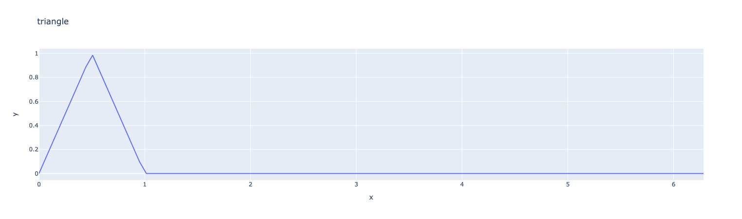
3.8. triangle

The triangle function is defined as $\text{triangle}(x)=1-\left|\chi_{[a,b]} \left(-1+2\frac{x-a}{b-a} \right) \right\| ], \quad x\in[a,b]$

ex=fpp.expr("triangle(x,0,1):x")
x=np.linspace(0,2*math.pi,100)
y=ex.evaluate("x",x)

fig = px.line(x=x, y=y, title="rectangle triangle(0,1)",labels={"x":"x","y":r'y'})
fig.show()

python

Results

3.9. sinwave

The sinwave function is a periodic function with a given period and amplitude.

ex=fpp.expr("sinewave(x,2,0.5):x")
x=np.linspace(0,2*math.pi,200)
y=ex.evaluate("x",x)

fig = px.line(x=x, y=y, title="sinewave(4*pi*x+0.5)",labels={"x":"x","y":r'y'})
fig.show()

python

Results

Manipulate Expressions

1. Create and evaluate expressions

1.1. Scalar expression

1.2. Vectorial expression

1.3. Matricial expression

2. Differentiation

2.1. Derivative of a vectorial expression

3. Special functions

3.1. function with multiple parameters

3.2. clamp

3.3. mapabcd

3.4. step1

3.5. smoothstep

3.6. pulse

3.7. rectangle

3.8. triangle

3.9. sinwave

4. Next steps