 .pdf
.pdf
Reduced Basis Methods
1. Model Order Reduction
1.1. Definition
1.1.1. Problem statement
Goal : Replicate input-output behavior of large-scale system \(\Sigma\) over a certain (restricted) range of
-
forcing inputs and
-
parameter inputs
Given large-scale system \(\Sigma_\mathcal{N}\) of dimension \(\mathcal{N}\), find a reduced order model \(\Sigma_N\) of dimension \(N << \mathcal{N}\) such that: The approximation error is small, i.e., there exists a global error bound such that :
-
\(\|u(\mu) - u_N (\mu)\| \leq \varepsilon_{\mathrm{des}}\), and \(|s(\mu) - s_N (\mu)| \leq \varepsilon^s_{\mathrm{des}} , \forall \mu \in D^{\mu}\).
-
Stability (and passivity) is preserved.
-
The procedure is computationally stable and efficient.
1.2. Motivation
Generalized Inverse Problem :
-
Given PDE(\(\mu\)) constraints, find value(s) of parameter \(\mu\) which:
-
(OPT) minimizes (or maximizes) some functional;
-
(EST) agrees with measurements;
-
(CON) makes the system behave in a desired manner;
-
or some combination of the above
-
-
Full solution computationally very expensive due to a repeated evaluation for many different values of \(\mu\)
-
Goal: Low average cost or real-time online response.
1.3. Methodologies
-
Reduced Basis Methods
-
Proper Orthogonal Decomposition
-
Balanced Truncation
-
Krylov Subspace Methods
-
Proper Generalized Decomposition
-
Modal Decomposition
-
Physical model reduction
-
…
|
Disclaimer on Model Order Reduction Techniques
|
1.4. Summary
Many problems in computational engineering require many or real-time evaluations of PDE(\(\mu\))-induced + input-output relationships.
Model order reduction techniques enable certified, real-time calculation + of outputs of PDE(\(\mu\)) + for parameter estimation, optimization, and control.
2. Reduced Basis Method
2.1. Problem Statement
A model order reduction technique that allows efficient and reliable reducedorder approximations for a large class of parametrized partial differentialequations (PDEs) in real-time or in the limit of many queries.
-
Comparison to other model reduction techniques:
-
Parametrized problems(material, constants, geometry,…)
-
A posteriori error estimation
-
Offline-online decomposition
-
Greedy algorithm (to construct reduced basis space)
-
-
Motivation :
-
Efficient solution of optimization and optimal control problems governed by parametrized PDEs.
-
2.1.1. Problem statement
Given a parameter \(\underbrace{\mu}_{\text{parameter}} \in \underbrace{D^\mu}_\text{parameter domain}\), evaluate \(\underbrace{s(\mu)}_\text{output} = L(\mu)^T \underbrace{u(\mu)}_\text{field variable}\) where \(u(\mu)\in\underbrace{X}_\text{FE space}\) satisfies a PDE \(A(\mu) u(\mu) = f(\mu)\).
Difficulties :
-
Need to solve \(\textit{PDE}_{FE}(\mu)\) numerous times at different values of \(\mu\),
-
Finite element space \(X\) has a large dimension \(\mathcal{N}\).
2.1.3. General Problem Statement
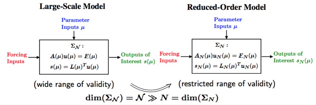
Given a system \(\Sigma_\mathcal{N}\) of large dimension N,
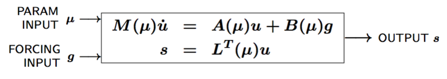
where
-
\(u(\mu, t) \in \mathbb{R}^{\mathcal{N}}\), the state
-
\(s(\mu, t)\), the outputs of interest
-
\(g(t)\), the forcing or control inputs
are functions of
-
\(\mu \in D\), the parameter inputs
-
\(t\), time
and the matrices \(M\), \(A\), \(B\), and \(L\) also depend on \(\mu\).
Construct a reduced order system \(\Sigma_N\) of dimension \(N \ll \mathcal{N}\),
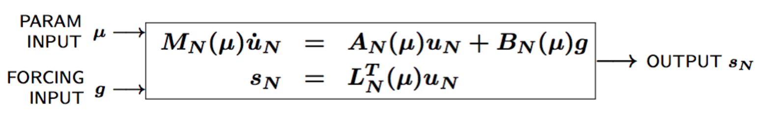
where \(u_N(\mu) \in \mathbb{R}^N\) is the reduced state.
We start by considering \(\dot{u} = 0\)
Full Model
\(\begin{align} A(\mu) u(\mu)& = & F(\mu)\\ s(\mu)&=&L^T(\mu) u(\mu) \end{align}\)
Reduced Model
\(\begin{align} A_N(\mu) u_N(\mu)& = & F_N(\mu)\\ s_N(\mu)&=&L^T_N(\mu) u_N(\mu) \end{align}\)
2.2. Key ingredients
2.2.1. Approximation
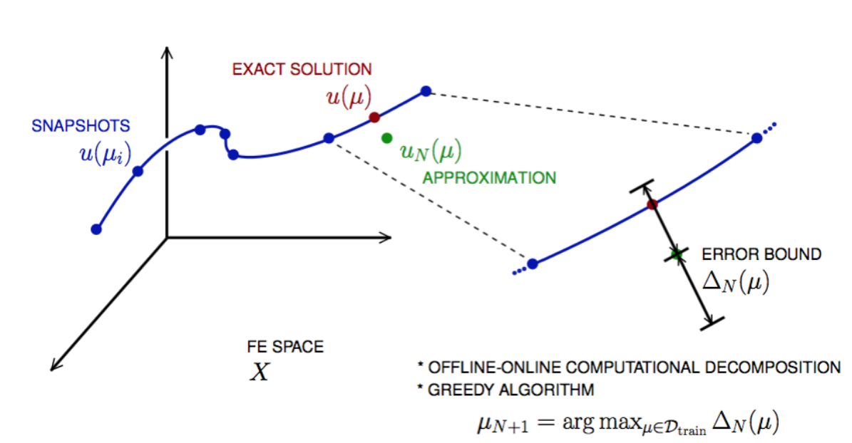
-
Take « snapshots » at different \(\mu\)-values: \(u(\mu_i), i = 1 \ldots N\), and let \(Z_N=[\xi_1,\ldots,\xi_N] \in \mathbb{R}^{\mathcal{N}\times N}\) where the basis/test functions, \(\xi_i\) « \(=\) » \(u(\mu_i)\), are orthonormalized
-
For any new \(\mu\), approximate \(u\) by a linear combination of the \(\xi_i\) \(u(\mu) \approx \sum_{i=1}^N u_{N,i}(\mu) \xi_i = Z_N u_N(\mu)\) determined by Galerkin projection, i.e.,
2.2.2. A posteriori error estimation
-
Assume well-posedness; \(A(\mu)\) positive and definite with a minimal eigenvalue \(\alpha_a :=\lambda_1 >0\), where \(A \xi=\lambda X \xi\) and \(X\) corresponds to the \(X\)-inner product, \((v, v)_X = \|v\|_X^2\)
-
Let \(\underbrace{e_N = u - Z_N\ u_N}_{\text{error}}\) , and \(\underbrace{r = F - A\ Z_N\ u_N}_{\text{residual}}, \forall \mu \in D^\mu\), so that \(A(\mu) e_N (\mu) = r(\mu)\)
-
Then (LAX-MILGRAM) for any \(\mu \in D^\mu\), \(\|u(\mu)- Z_N u_N(\mu) \|_X \leq \frac{\|r(\mu)\|_{X'}}{\alpha_{LB}(\mu)} =: \Delta_N(\mu)\), \(|s(\mu)-s_N(\mu)| \leq \|L\|_{X'} \Delta_N(\mu) =: \Delta^s_N(\mu)\) where \(\alpha_{LB}(\mu)\) is a lower bound to \(\alpha_a(\mu)\), and \(\|r\|_{X'}=r^T X^{-1} r\).
2.2.3. Offline-Online decomposition
How do we compute \(u_N\), \(s_N\), \(\Delta_N^s\) for any \(\mu\) efficiently online ?
We assue \(A(\mu) = \displaystyle\sum_{q=1}^Q \theta^q(\mu)A^q\) where
-
\(\theta^q(\mu)\) are parameter depandent coefficients,
-
\(A^q\) are parameter independent matrices
so that \(A_N(\mu) = Z_N^T A(\mu)Z_N = \displaystyle \sum_{q=1}^Q \theta^q(\mu)\underbrace{Z_N^T A^q Z_N}_\text{parameter independant}\)
Since all required quantities can be decomposed in this manner, we can split the process in two phases :
-
OFFLINE : Form and store \(\mu\)-independant quantities at cost \(O(\mathcal{N})\),
-
ONLINE : For any \(\mu\in D^\mu\), compute approximation and error obunds at cost \(O(QN^2+N^3)\) and \(O(Q^2N^2)\).
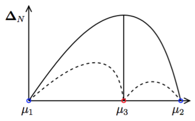
2.2.4. Greedy Algorithm
How do we choose the sample points \(\mu_i\) (snapshots) optimally ?
Given \(Z_{N=2} « = » [u(\mu_1), u(\mu_2)]\), we choos \(\mu_{N+1}\) as follows
and \(Z_{N+1} := [u(\mu_1),\cdots, u(\mu_{N+1})\).
-
Key : \(\Delta_N(\mu)\) is sharp and inexpensive to compute (online)
-
Error bound gives « optimal » samples, so we get a good approximation \(u_N(\mu)\).
2.3. Summary
2.3.1. Reduced Basis Opportunities Computational Opportunities
-
We restrict our attention to the typically smooth and low-dimensional manifold induced by the parametric dependence.
\(\Rightarrow\) Dimension reduction -
We accept greatly increased offline cost in exchange for greatly decreased online cost.
\(\Rightarrow\) Real-time and/or many-query context
2.3.2. Reduced Basis Relevance
Real-Time Context (control,\(\ldots\)): \(\begin{align} \mu & \rightarrow & s_N(\mu), \Delta^s_N(\mu) & \\ t_0 \text{(« input »)} & & & t_0+\delta t_{\mathrm{comp}} (\text{« response »}) \end{align}\)
Many-Query Context (design,\(\ldots\)): \(\begin{align} \mu_j & \rightarrow & s_N(\mu_j), \Delta^s_N(\mu_j),\quad j=1\ldots J \\ t_0 & & t_0+\delta t_{\mathrm{comp}} J\quad (J \rightarrow \infty) \end{align}\)
\(\Rightarrow\) Low parginal (real-time) and/or low average (many-query) cost.
2.3.3. Reduced Basis Challenges
-
A Posteriori error estimation
-
Rigorous error bounds for outputs of interest
-
Lower bounds to the stability « constants »
-
-
Offline-online computational procedures
-
Full decoupling of finite element and reduced basis spaces
-
A posteriori error estimation
-
Nonaffine and nonlinear problems
-
-
Effective sampling strategies
-
High parameter dimensions
-
2.3.4. Reduced Basis Outline
-
Affine Elliptic Problems
-
(non)symmetric, (non)compliant, (non)coercive
-
(Convection)-diffusion, linear elasticity, Helmholtz
-
-
Affine Parabolic Problems
-
(Convection)-diffusion equation
-
-
Nonaffine and Nonlinear Problems
-
Nonaffine parameter dependence, nonpolynomial nonlinearities
-
-
Reduced Basis (RB) Method for Fluid Flow
-
Saddle-Point Problems (Stokes)
-
Navier-Stokes Equations
-
-
Applications
-
Parameter Optimization and Estimation (Inverse Problems)
-
Optimal Control
-