 .pdf
.pdf
Fluid Structure Interaction
The Fluid Structure models are formed from the combination of a Solid model and a Fluid model.
1. Definitions
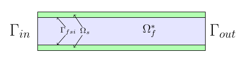
Let \(I=[t_i,t_f[\) be the time interval, and \(t\in I\) denotes the time. \(\Omega^t_f\) is the fluid domain, the exponent \(\phantom{}^t\) indicates that the domain changes over time, we work in an Eulerian setting. We denote \(\Omega^*_s\) the solid wall which is set in a Lagrangian setting. We also introduce \(\Omega_f^*\) the reference fluid domain, which can be chosen as \(\Omega_f^* \equiv \Omega_f^{t_i}\) where \(t_i\) is the initial time.
1.1. Variables, symbols and units
Notation |
Quantity |
Unit |
\(\boldsymbol{u}_f\) |
fluid velocity |
\(m.s^{-1}\) |
\(\boldsymbol{\sigma}_f\) |
fluid stress tensor |
\(N.m^{-2}\) |
\(\boldsymbol{\eta}_s\) |
displacement |
\(m\) |
\(\boldsymbol{F}_s\) |
deformation gradient |
dimensionless |
\(\boldsymbol{\Sigma}_s\) |
second Piola-Kirchhoff tensor |
\(N.m^{-2}\) |
\(\mathcal{A}_f^t\) |
Arbitrary Lagrangian Eulerian ( ALE ) map |
dimensionless |
2. ALE Map
To couple the fluid and the solid dynamics, we need to formulate the fluid equations in Lagrangian coordinates. To this end, we introduce the Arbitrary Lagrangian Eulerian (ALE) framework which allows to go from the Eulerian to the Lagrangian frame and vice versa, and more specifically we define the ALE map.
This map give us the position of \(x\), a point in the deformed domain at time \(t\) from the position of \(x^*\) in the initial configuration \(\Omega^*\). Figure 1 displays a schematic of the fluid structure interaction (FSI) and the action of the ALE map \(\mathcal{A}_{}^t\).
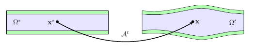
\(\mathcal{A}^t\) is a homeomorphism, i.e. a continuous and bijective application we can define as
where \(\mathbf{x}\) is the position in \(\Omega_f^t\) of the point which was at \(\mathbf{x}^*\) in \(\Omega_f^*\).
We denote also \(\forall \mathbf{x}^* \in \Omega^*\), the application :
We can then define the Lagrangian derivative
where \(\boldsymbol{u}\) is a vector field and \(\boldsymbol{w}\) is the velocity of the mesh displacement defined as follows
Variables defined in the reference frame are denoted as follows \(\hat{\boldsymbol{u}} = \boldsymbol{u} \circ \mathcal{A}_{}^t\)
And finally we denote
and
3. Example of fluid and structure models
Consider a laminar incompressible flow, the velocity and pressure \((\boldsymbol{u}_f,p_f)\) are then given by the equations
with
and
and where \(\boldsymbol{f}_t\) is the volumic force density, \(\rho_f\) the blood density and \(\mu_f\) the blood viscosity.
Consider now a nearly incompressible hyperelastic structure. We use, in this case, a displacement-pressure formulation following a Saint Venant-Kirchhoff material law. The displacement and pressure \((\boldsymbol{\eta}_s, p_s)\) equations read:
where \(\lambda_s\), \(\mu_s\) are the Lamé coefficients defined as \(\lambda_s = \frac{E_s \nu_s}{ (1+\nu_s)(1-2\nu_s)} \quad , \quad \mu_s = \frac{E_s}{2(1+\nu_s)},\) \(\rho_s (\textrm{ kg}\,\textrm{mm}^3)\) is the structure density, \(E_s (\textrm{ kg}\,\textrm{mm}^{-1}\,\textrm{s}^{-2})\) is the Young modulus and \(nu_s\) is the Poisson coefficient.
More information are available in the theoretical description of the fluid equations, and the structure equations.
The solution of this model are \((\mathcal{A}^t, \boldsymbol{u}_f, p_f, \boldsymbol{\eta}_s)\).
4. Coupling conditions
In order to have a complete fluid-structure model, we need to add to the solid model and the fluid model equations some coupling conditions :
\(\boldsymbol{(1)}, \boldsymbol{(2)}, \boldsymbol{(3)}\) are the fluid-struture coupling conditions, respectively velocities continuity, constraint continuity and geometric continuity.
4.1. Fluid structure coupling conditions with 1D reduced model
In the case of a 2D fluid and 1D structure, we need to modify the original ones \(\boldsymbol{(1)},\boldsymbol{(2)}, \boldsymbol{(3)}\) by
5. Discretization
Regarding the space discretization, we use the finite element method to discretize the model described above. We use continuous piecewise polynomials of order \(k+1\) for the velocity and order \(k\) for the pressure in the fluid and we use continuous piecewise polynomials of order \(k\) for the displacement.
| The ALE map would be descretized with the same polynomial order as the displacement. |
Regarding the time discretization, we can use for the fluid a \(BDF_2\) scheme and for the solid we use the Newmark scheme, both are second order in time.
The algebraic representation of the fluid and solid model are solved using iterative methods preconditioned with algebraic-factorization type preconditioners enabling fast solves. The fluid-structure interaction coupling is handled with a Picard method that iterates between the fluid and the solid models until the relative increment between two non-linear iterations reaches a given tolerance.
The FSI solution strategy follows a partitioned method solving at time \(t^n\) alternatively for the solid displacement \(\boldsymbol{\eta}_s^n\) and then the fluid velocity and pressure \(\boldsymbol{u}_f^{n}, p_f^n\) until convergence.
Different coupling strategies (semi-implicit and semi-explicit) can be set between fluid and the structure:
-
using a Dirichlet-Neumann scheme
-
using a Robin-Robin coupling scheme between the fluid and the structure.
-
using a Generalized Robin-Neumann scheme
| The list needs to be updated |
6. Coupling strategies
Discrete coupling conditions must mimic the continuous coupling conditions that impose velocity, stress and geometric continuity on the FSI interface.
FSI coupling conditions can be practically enforced in different ways. A key element determining the numerical scheme to be used is the added-mass effect. This phenomenon depends on the ratio \(\frac{\rho_s}{\rho_f}\) and refers to the different acceleration that a body immersed in a fluid experiences, as opposed to the acceleration it would experience in vacuum. This effect is explained by imagining that, as it moves, the solid carries with it a certain volume of fluid, and the higher the fluid density, the stronger the added mass. The added-mass effect is strong when fluid and solid densities are approximately equal.
Initially, when FSI simulations were carried out for aerodynamic purposes, this effect was negligible and a Dirichlet-Neumann approach was employed; lately, FSI modeling started employing denser fluids, and numerical schemes that are independent from added mass effects became necessary: two examples are Robin-Robin and Generalized Robin-Neumann schemes. They are all explicit schemes.
6.1. Dirichlet-Neumann
Dirichlet-Neumann coupling strategy is the easiest and directest one. It discretizes the FSI coupling conditions as follows: at the \(n\)-th time iteration, on the fluid sub-problem the following conditions are imposed
They are the discretized Dirichlet prescription on the velocity suggested by the coupling conditions.
On the solid sub-problem, instead, the Neumann condition on the stresses' continuity is imposed in a discrete form
6.2. Robin-Robin
Robin-Robin (RR) coupling strategy imposes coupling conditions in Robin form, in two steps: at the \(n\)-th time iteration, on the solid sub-problem the following conditions are imposed
where
The right-hand side depends only on quantities coming from the \((n-1)\)-th time iteration.
Once the solid sub-problem has been solved, one uses \(\mathbf{u}_s^n \) to impose on the fluid sub-problem:
Here, \(\gamma\) is a penalization parameter to be chosen.
It should be noticed that in (RR) stability and accuracy are subject to a CFL-condition: hyperbolic-type CFL, for which \(\Delta t = \mathcal{O}(h)\), is sufficient to have stability, but parabolic-type CFL, for which \(\Delta t = \mathcal{O}(h^2)\), is necessary to have optimal accuracy.
6.3. Generalized Robin-Neumann
This coupling strategy, at the \(n\)-th time iteration, imposes on the fluid sub-problem:
where
and \(\mathbf{B}\) is a self-adjoint operator coming from a mass lumping procedure. The fluid-sided condition is called generalized Robin because of \(\bf{B}\) that multiplies fluid and solid velocities.
On the solid sub-problem, the following discrete Neumann condition is imposed
Also in this case there are CFL-type constraints that link space and time discretization steps: under parabolic-type CFL condition, stability is guaranteed; however, if adequate extrapolation techniques are employed, stability can be obtained under weaker requirements.
These succint explanations were taken from the articles:
-
Erik Burman, Miguel Angel Fernández. Explicit strategies for incompressible fluid-structure inter- action problems: Nitsche type mortaring versus Robin-Robin coupling. International Journal for Numerical Methods in Engineering, Wiley, 2014, 97 (10), pp.739–758. <10.1002/nme.4607>. <hal- 00819948v2> hal.inria.fr/hal-00819948v2
-
Miguel Angel Fernández, Jimmy Mullaert, Marina Vidrascu. Generalized Robin-Neumann explicit coupling schemes for incompressible fluid-structure interaction: stability analysis and numerics. International Journal for Numerical Methods in Engineering, Wiley, 2015, 101 (3), pp.199-229. <10.1002/nme.4785>. <hal-00875819> hal.inria.fr/hal-00875819