 .pdf
.pdf
Post-Processing and Visualization
1. Introduction
Once the PDE is solved we usually would like to visualize the solution and possibly other data or fields associated with the problem. Feel++ provides a very powerful framework for post-processing allowing to:
-
visualize time-based data,
-
visualize high order functions,
-
visualize traces,
-
use standard visualization tools such as Paraview, Ensight and Gmsh.
To achieve this, Feel++ defines a so-called Exporter object.
2. General principles
The library Feel++ itself does not have any visualization capabilities.
However, it provides tools to export both scalar and vector fields into two formats: EnSight and Gmsh.
The EnSight format can be read by the visualization software EnSight or, for instance, by the open source package Paraview.
The choice of format depends on several factors, some of them being the robustness/capabilities of the visualization packages associated and the type of data to be plotted.
For first (at most second) degree piecewise polynomials defined in straight edge/faces meshes, ParaView (or any other software that reads the EnSight format) is a very good choice. A trick to use Paraview (or any other visualization software that plots first order geometrical and finite elements) to visualize high degree polynomials in curved meshes, is to use an interpolation operator built on high order nodes associated with the polynomial space, see~\cite gpena_cprudhomme_acomen. However, for high degree polynomials or meshes with curved elements, Gmsh is prefered due to its adaptive visualization algorithm for this type of finite/geometrical element.
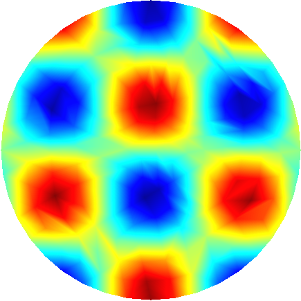
To illustrate both approaches in visualizing high degree polynomials in curved meshes, we plot, in the Figures below, the nodal projection of the function \(f(x,y)=\cos(5x) \sin(5y)\) in the unit circle onto several function spaces. Notice the improved rendering of the projection using high degree polynomials instead of linear projections in a finer mesh. We remark also that the difference between the two approaches fades away as we increase the degree of the polynomials and the order of the geometrical elements. However, the additional cost of building the piecewise first order finite element space associated with the finer mesh, the calculation of the projection onto this space and the smoothness of the graphics makes Gmsh’s approach more appealing to visualize this type of finite elements. We highlight that these algorithms are available for meshes composed only of simplices or quadrilaterals, in 1D, 2D and 3D.
Order 1 |
Order 2 |
P2isoP1 |
Order 3 |
P3isoP1 |
Order 4 |
P4isoP1 |
Order 5 |
P5isoP1 |
|
|
|
|
|
|
|
|
|
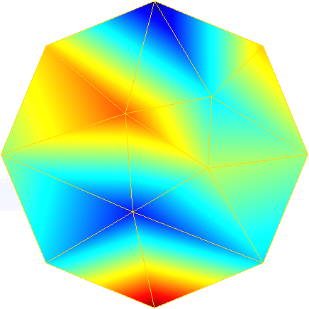
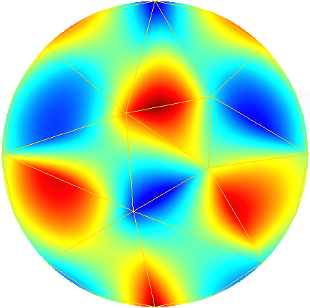
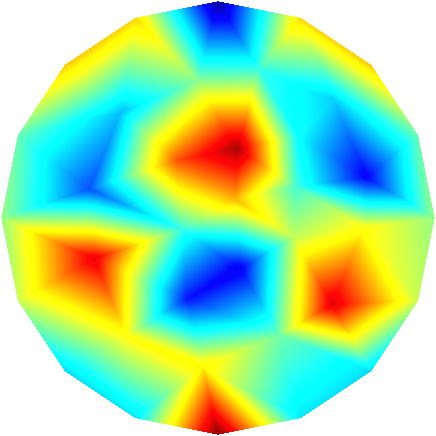
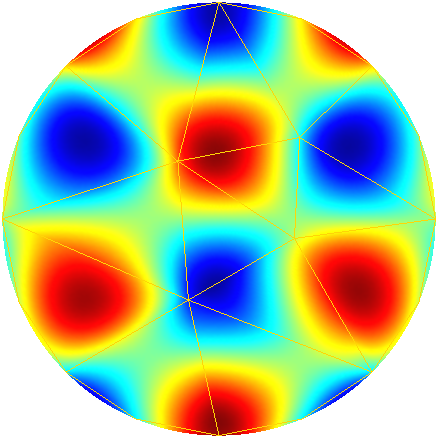
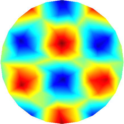
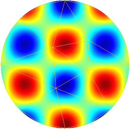
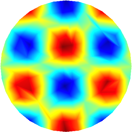
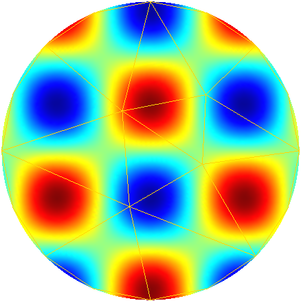
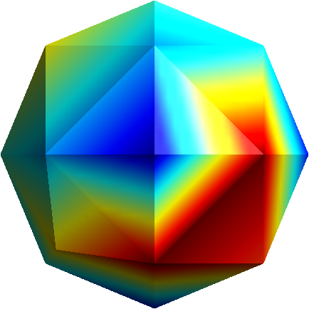
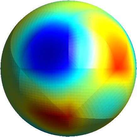
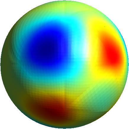
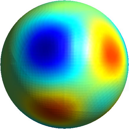
To further illustrate the capabilities of the Feel’s exporter to Gmsh, we plot in Figures 1D and 3D functions defined on the unit sphere.
Order 1 |
Order 2 |
Order 3 |
Order 4 |
|
|
|
|
3. Visualization
We would like to visualize the function \(u=\sin(\pi x)\) over \(\Omega= \{ (x,y) \in \mathbb{R}^2 | x^2 + y^2 < 1 \}\) \(\Omega\) is approximated by \(\Omega_h\).
To define \(\Omega\) and \(u\) the code reads mesh
  auto exhi = exporter( _mesh=mesh, _name="exhi" );
  auto exlo = exporter( _mesh=meshp1, _name="exlo" );
  auto exhilo = exporter( _mesh=lagrangeP1(_space=Xh)->mesh(),_name="exhilo");

  int max = 10; double dt = 0.1;
  double time = 0;
  for (int i = 0; i<max; i++)
  {
    exhilo->step( time )->add( "vhilo", v );
    exlo->step( time )->add( "vlo", v );
    exhi->step( time )->add( "vhi", v );
    time += dt;
    exhi->save();
    exlo->save();
    exhilo->save();
  }
We start with an Exporter object that allows to visualize the \(P_1\) interpolant of \(u\) over \(\Omega\).
4. ExporterReference Reference
4.1. Options
exporter.format
-
Type: multiple choice
string -
Values:
gmsh,ensight,ensightgold -
Default value: ensightgold
-
Action:
exporter.formatdefines the format to save Feel++ data into.
exporter.geometry
-
Type: multiple choice
string -
Values:
change_coords_only,change,static -
Default value: change_coords_only
-
Action:
exporter.geometrytells to the exporter if the mesh changes over time steps : no changes (static)coordinates only (change_coords_only)or remeshed (changes)
exporter.fileset
-
Type:
bool -
Values:
0,1 -
Default value:
0 -
Action:
exporter.fileset=0 save one file per timestep per subdomain, whereasexporter.fileset=1 use one file per subdomain to store all time steps.
This option,
exporter.fileset=1, reduces tremendously the number of files generated for transient simulations.
exporter.prefix
-
Type:
string -
Default Value:
<empty string> -
Action:
exporter.prefixdefines the prefix to be user by the exporter. It is especially useful when using multiple exporters and avoid name collision.
exporter.directory
-
Type:
string -
Default Value: results
-
Action:
exporter.directorytells where to export the results
4.1.1. Ensight Gold specific options
exporter.ensightgold.use -sos
-
Type:
bool -
Action: if
exporter.ensightgold.use-sos=0 multiple case files are handle in first case file else the sos file is used to handle multiple case files
exporter.ensightgold.save -face
-
Type:
bool -
Action: if
exporter.ensightgold.save-face=1, the exporter saves mesh and fields on marked faces