.pdf
.pdf
Diffusion and Uptake into a Spherical Cell
We took this example from : [Socrates_Dokos_(auth.)]_Modelling_Organs,_Tissues(z-lib.org) .
1. Description
\(\quad\)In this example, we will build a diffusion and uptake into a spherical cell model. We will use Fick’s laws of diffusion.
\(\quad\) Fick’s second law describes the transient changes of concentration with time, and is written mathematically as a PDE in the concentration variable c:
with \(D\) the diffusion coefficient of the substance in a given medium in SI units of \(m^{2}s^{-1}\). The typical values for \(D\) are \([ 0.6 \times 10^{-9}, 2 \times 10^{-9}\)] \(m^{2}s^{-1}\) for individual ions and \([ 10^{-11}, 10^{-10}\)] \(m^{2}s^{-1}\) for biological molecules.
We obtain an equation similar to heat transfert. Thus we will use the toolbox heat.
For the Boundary Conditions, we have the typical value for cell surface: \(-0,0005c \ mol\ s^{-1}m^{-2}\) where \(c\) is the nutriment concentration in \(mM\)
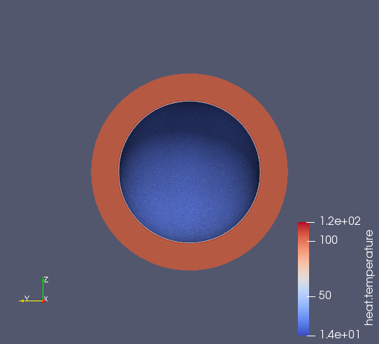
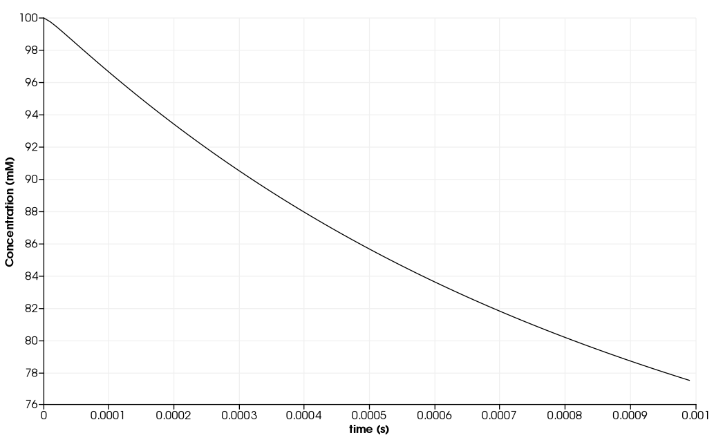
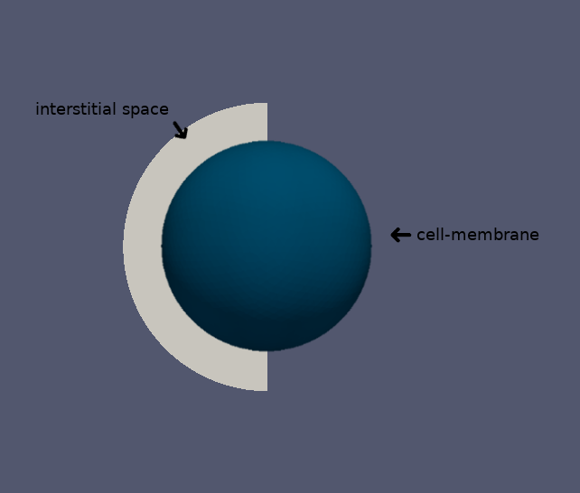
\(\quad\) We consider a spherical cell of radius \(50 \mu m\) taking a nutrient from the interstitial space and metabolising it. The initial concentration in the interstitial space is \(100 mM\), we try to find the concentration of nutrient \(0.5 \mu m\) from the cell surface as a function of the time.
2. Input
As we have this value \(-0,0005c \ mol\ s^{-1}m^{-2}\) for the boundary condition, we use Robin condition for the bondary condition:
and for thr PDE:
We will use those inputs:
Name |
Description |
Values |
Units |
\(D\) |
diffusion coefficient |
\(5 \times 10^{-11}\) |
\(m^{2}s^{-1}\) |
\(r_{cell}\) |
cell radius |
\(50 \times 10^{-6}\) |
\(m\) |
\(r_{exterior}\) |
exterior radius |
\(70 \times 10^{-6}\) |
\(m\) |
\(H\) |
uptake through the cell surface |
\(5 \times 10^{-4}\) |
\(mol\ s^{-1}\ m^{-2}\) |
\(G\) |
in cell concentration |
\(0\) |
\(mM\) |
Here we suppose that the concentration inside the cell is equal to 0, but we can change it.
3. Data files
The case data files are available in Github here
3.1. Json file
3.1.1. Names
A model JSON file starts by giving names (long and short).
"Name": " Diffusion and Uptake into a Spherical Cell", (1)
"ShortName":"Cell",(2)
| 1 | Name of the example, usually printed on-screen and in log files during simulations |
| 2 | Short name of the example, it is used to create directories to store the results of the simulation of the model |
3.1.2. Materials
This section of the Model JSON file defines material properties linking the Physical Entities in the mesh data structures to these properties.
"Materials":
    {
        "fluid":(1)
        {
	    "markers":"fluid", (1)
            "rho":"1", (2)
            "mu":"0", (2)
            "k":"5e-11", (3)
            "Cp":"1" (2)
        }
}| 1 | gives the name of the physical entity (here Physical Surface) associated to the Material. |
| 2 | \(\rho\) and \(C_p\) equal to 1 and \(\mu\) equals to 0 to have the similarity between the heat transfert equation and Fick’s law of diffusion. |
| 3 | here \(k\) take the role of \(D\). |
3.1.3. Boundary Conditions
This section of the Model JSON file defines the boundary conditions.
"BoundaryConditions":
    {
        "temperature": (1)
        {
             "Robin": (2)
            {
                "cell-membrane": (3)
                {
                  "expr1":"5e-4", (4)
                  "expr2":"0" (5)
                }
            }
        }
},| 1 | the field name of the toolbox to which the boundary condition is associated |
| 2 | the type of boundary condition to apply, here Robin |
| 3 | the physical entity (associated to the mesh) to which the condition is applied |
| 4 | expr1 is for the \(H\) expression |
| 5 | expr2 is for the \(G\) expression |
3.1.4. Post Process
"PostProcess": (1)
    {
      	"Exports": (2)
      	{
              "fields":["temperature","pid"] (3)
      	},
         "Measures": (4)
        {
            "Points": (5)
            {
                "pointA": (6)
                {
                    "coord":"{5.05e-5, 0,0}", (7)
                    "fields":"temperature" (8)
                }
            }
        }
}| 1 | the name of the section |
| 2 | the Exports identifies the toolbox fields that have to be exported for visualisation |
| 3 | the list of fields to be exported |
| 4 | the Mesures identifies the toolbox |
| 5 | the type of area to be measured, here Point |
| 6 | the name of the Point, here "pointA" |
| 7 | the coordinates of the point "pointA" |
| 8 | the type of measure to do, here temperature |
3.2. CFG file
The Model CFG (.cfg) files allow to pass command line options to Feel++ applications. In particular, it allows to
-
setup the mesh
-
define the solution strategy and configure the linear/non-linear algebraic solvers.
The Cfg file used is
directory=Cell3DExport (1)
case.dimension=3 (2)
[heat] (3)
mesh.filename=$cfgdir/cellule3d.geo (4)
gmsh.hsize=5e-7#0.01#0.05 (5)
filename=$cfgdir/cellule3d.json (6)
initial-solution.temperature=100 (7)
reuse-prec=1 (8)
pc-type=gamg (9)

[heat.bdf] (10)
order=2 (11)

[ts] (12)
time-step=1e-5 (13)
time-final=1e-3 (14)
restart.at-last-save=true (15)
| 1 | the directory where the results are exported |
| 2 | the dimension of the application, by default 3D |
| 3 | toolbox prefix |
| 4 | the geometric file |
| 5 | the mesh step |
| 6 | the associated Json file |
| 7 | the initial solution: here the temperature take the role of the concentration |
| 8 | to reuse the precedent solution |
| 9 | the chosen method for pre-conditionnement |
| 10 | heat.bdf |
| 11 | heat.bdf order |
| 12 | time setup |
| 13 | time step |
| 14 | time final |
| 15 | restart at last save |
We didn’t configure the solver, cause in this case, the system is linear, and by default the solver chosen is the linear one.