Sensor

1. Introduction

Presentation of the basic for force measurement with strain gauges.

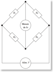
A strain gauge is a device used to measure strain on an object. The most common type of strain gauge consists of an insulating flexible backing which supports a metallic foil pattern. The gauge is attached to the object by a suitable adhesive. As the object is deformed, the foil is deformed, causing its electrical resistance to change. This resistance change, usually measured using a Wheatstone bridge, is related to the strain by the quantity known as the gauge factor.

CAD representation of a strain gauge
Representation of a strain gauge
Strain gauge

2. Running the case

2.1. Command line

The command line to run this case is

!mpirun -np 4 feelpp_toolbox_solid --case "github:{repo:toolbox,path:examples/modules/csm/examples/sensor}"

The report of the execution of the command above is available here.

2.2. Python interface

We start with the Feel++ environment.

from feelpp import *
from feelpp.toolboxes.core import *
from feelpp.toolboxes.solid import *

# create the application
# create a feelppdb subdirectory where the results are stored
app = Environment(['feelpp_toolbox_solid'], opts= toolboxes_options("solid"),config=localRepository(""))

Next we download the study configuration and simulate it

sensorcfg=feelpp.download("github:{repo:toolbox,path:examples/modules/csm/examples/sensor/}", worldComm=app.worldCommPtr())[0] (1)
sensorcfg+='/sensor.cfg' (2)
if os.path.exists(sensorcfg): (3)
  app.setConfigFile(sensorcfg) (4)
  s = solid(dim=3) (5)
  # get displacement and von-mises measures from the model
  ok,meas=simulate(s) (6)
  if ok:
    # export in paraview format
    s.exportResults() (7)

1	download the configuration file
2	add the configuration file to the study
3	check if the configuration file exists
4	set the configuration file
5	create the solid mechanics model
6	simulate the model and get the resulting measures from the PostProcessing section
7	export the results

Results

[ Starting Feel++ ] application feelpp_toolbox_solid version 0.1 date 2022-Nov-07
 . feelpp_toolbox_solid files are stored in /scratch/jupyter/feelppdb/np_1
 .. logfiles :/scratch/jupyter/feelppdb/np_1/logs
Reading /scratch/jupyter/feelppdb/downloads/sensor/sensor.cfg...
solid(3,1)
[modelProperties] Loading Model Properties : "/scratch/jupyter/feelppdb/downloads/sensor/sensor.json"
[loadMesh] Loading Gmsh compatible mesh: "/scratch/jupyter/feelppdb/downloads/solid/meshes/sensor.msh"
[loadMesh] Loading Gmsh compatible mesh: "/scratch/jupyter/feelppdb/downloads/solid/meshes/sensor.msh" done
============================================================

time simulation: 0.05s/0.61s with step: 0.05
============================================================

 0 solid SNES Function norm 4.324537e+02
 1 solid SNES Function norm 3.894843e+02
  Linear solve converged due to CONVERGED_RTOL iterations 9
 2 solid SNES Function norm 3.511776e+02
  Linear solve converged due to CONVERGED_RTOL iterations 9
 3 solid SNES Function norm 3.103868e+02
  Linear solve converged due to CONVERGED_RTOL iterations 9
 4 solid SNES Function norm 2.657841e+02
  Linear solve converged due to CONVERGED_RTOL iterations 9
 5 solid SNES Function norm 2.165992e+02
  Linear solve converged due to CONVERGED_RTOL iterations 9
 6 solid SNES Function norm 1.624799e+02
  Linear solve converged due to CONVERGED_RTOL iterations 9
 7 solid SNES Function norm 1.621619e+02
  Linear solve converged due to CONVERGED_RTOL iterations 9
 8 solid SNES Function norm 6.411767e-03
  Linear solve converged due to CONVERGED_RTOL iterations 11
 9 solid SNES Function norm 6.553165e-06
  Linear solve converged due to CONVERGED_RTOL iterations 10
 10 solid SNES Function norm 9.171302e-10
  Linear solve converged due to CONVERGED_RTOL iterations 12
============================================================

time simulation: 0.1s/0.61s with step: 0.05
============================================================

 0 solid SNES Function norm 4.056531e+02
 1 solid SNES Function norm 3.653160e+02
  Linear solve converged due to CONVERGED_RTOL iterations 9
 2 solid SNES Function norm 3.265140e+02
  Linear solve converged due to CONVERGED_RTOL iterations 9
 3 solid SNES Function norm 2.843344e+02
...

time simulation: 0.44999999999999996s/0.61s with step: 0.05

3. Data files

The case data files are available in Github here

CFG file - [Edit the file]
JSON file - [Edit the file]

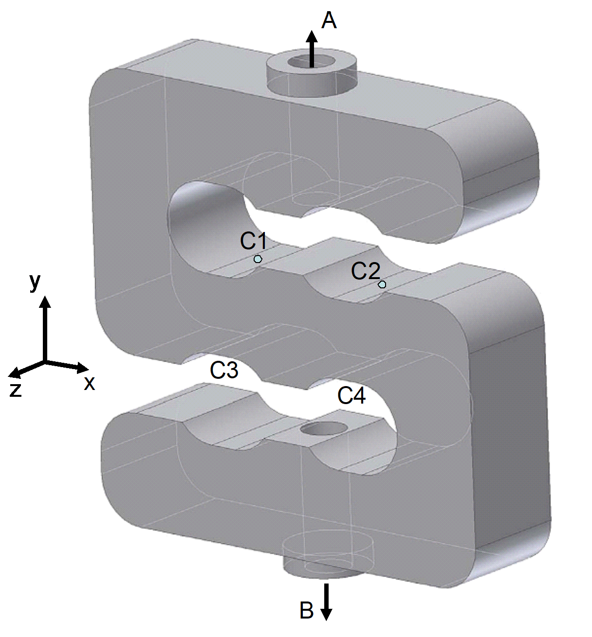
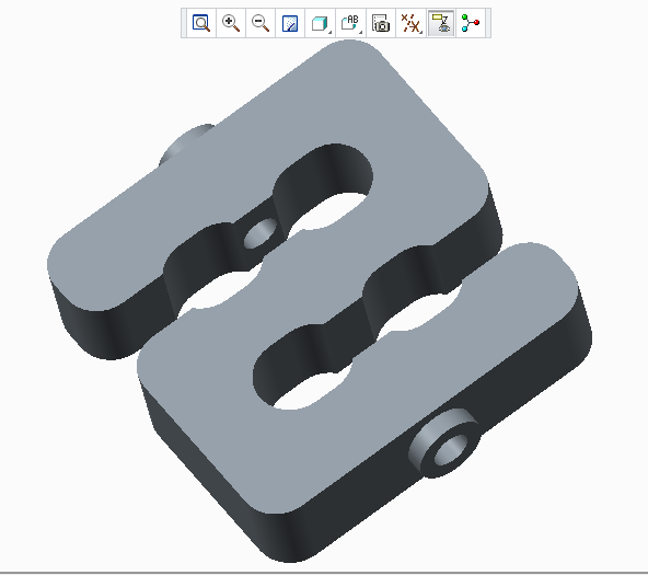
4. Model/Geometry

The first step is to create the model of the object, which we can simply do in the Creo Parametric program. With this program was the fastest and easiest way to create the model.

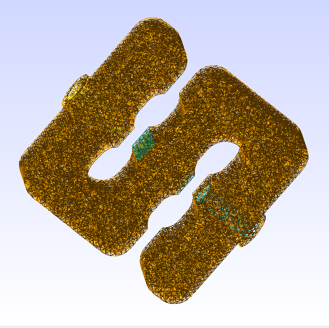
The finished geometry (Creo) and the meshed model (Gmsh):

CAD representation of a strain gauge
Mesh representation of a strain gauge

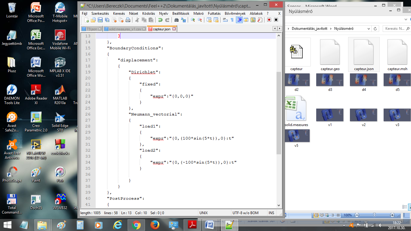
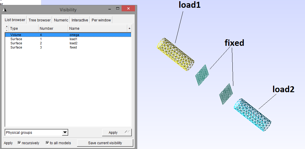
5. Materials and boundary conditions

5.1. Materials

The beam is made of steel, so we need to use the following data:

\(E = 205 GPa -> 205e3 N/mm^2\)
\(nu = 0.3\)
\(rho = 7850 kg/m^3 -> 7850e-9 kg/mm^3\)

5.2. Boundary conditions

The object is fixed in the middle. Holes have opposite sinusodal forces.

CAD representation of a strain gauge
Mesh representation of a strain gauge

6. Results

The result were run in time (half whole period, but on the pictures can be seen only a quarter period).

import pandas as pd
df=pd.DataFrame(meas)
print(df.head())

# prepare for plotting
import plotly.graph_objects as go

Results

Paraview files are in /scratch/jupyter/feelppdb/np_1/np_1/solid.exports
   Statistics_disp_max  Statistics_disp_mean_0  Statistics_disp_mean_1  \
0             0.000000                0.000000                0.000000
1             0.423963                0.000030                0.000024
2             0.823267                0.000058                0.000047
3             1.147965                0.000077                0.000067
4             1.425199                0.000096                0.000084

   Statistics_disp_mean_2  Statistics_disp_min  Statistics_von-mises_max  \
0                0.000000             0.000000                  0.000000
1               -0.000017            -0.424049                986.291965
2               -0.000033            -0.823410               1926.227644
3               -0.000046            -1.148120               2715.268042
4               -0.000058            -1.425366               3380.035626

   Statistics_von-mises_mean  Statistics_von-mises_min  time
0                   0.000000                  0.000000  0.00
1                  76.661865                  0.000664  0.05
2                 149.031439                  0.003552  0.10
3                 208.581334                  0.002816  0.15
4                 259.019382                  0.004327  0.20

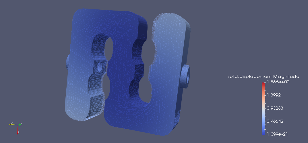
6.1. Displacement

displacement at \(t=0.1s\)
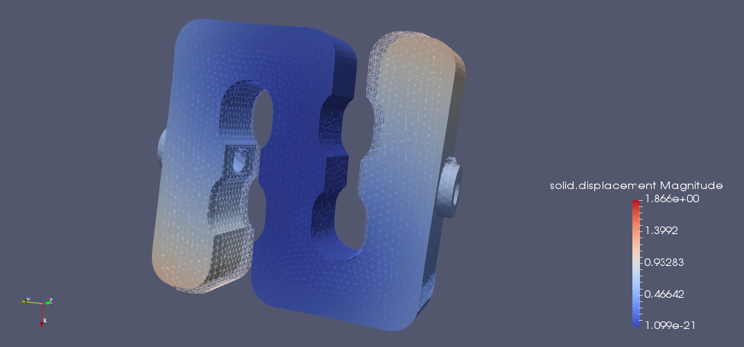
displacement at \(t=0.2s\)
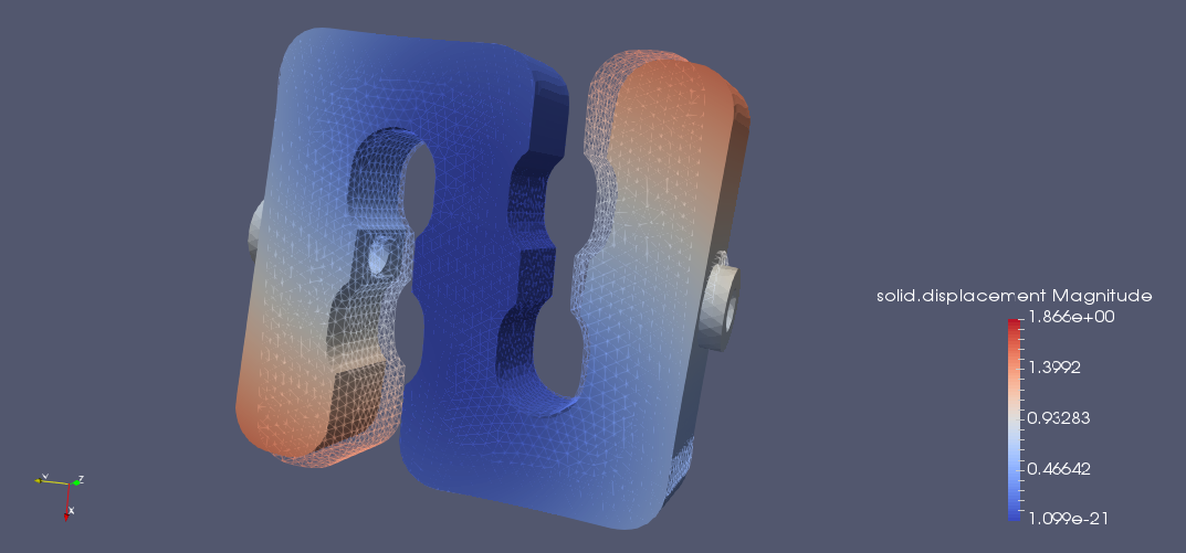
displacement at \(t=0.3s\)
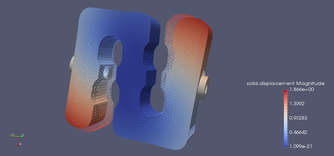
displacement at \(t=0.4s\)
displacement at \(t=0.5s\)

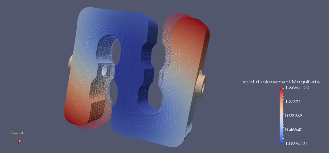
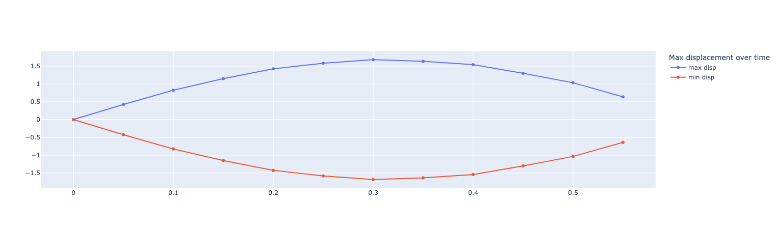
Plot the max of the displacement over time

fig = go.Figure()
fig.add_trace(go.Scatter(x=df["time"], y=df["Statistics_disp_max"], name="max disp"))
fig.add_trace(go.Scatter(x=df["time"], y=df["Statistics_disp_min"], name="min disp"))
fig.update_layout(legend_title_text='Max displacement over time')
fig.show()

Results

minmaxdisp

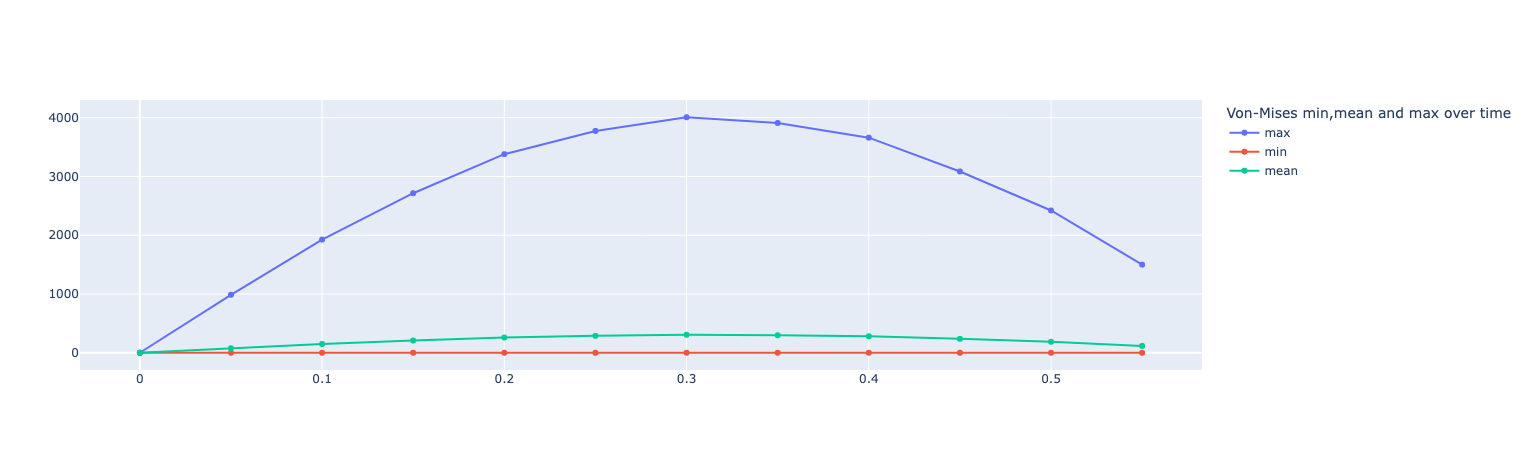
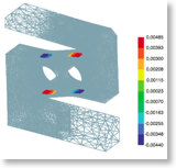
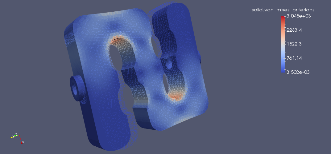
6.2. Von-Mises Criterions

Von-Mises criterion at \(t=0.1s\)
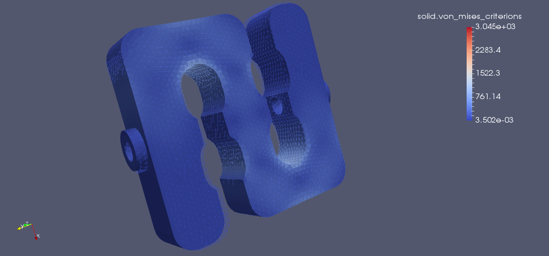
Von-Mises criterion at \(t=0.2s\)
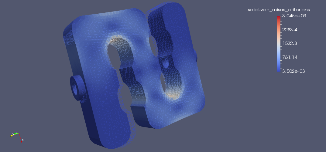
Von-Mises criterion at \(t=0.3s\)
Von-Mises criterion at \(t=0.4s\)
Von-Mises criterion at \(t=0.5s\)

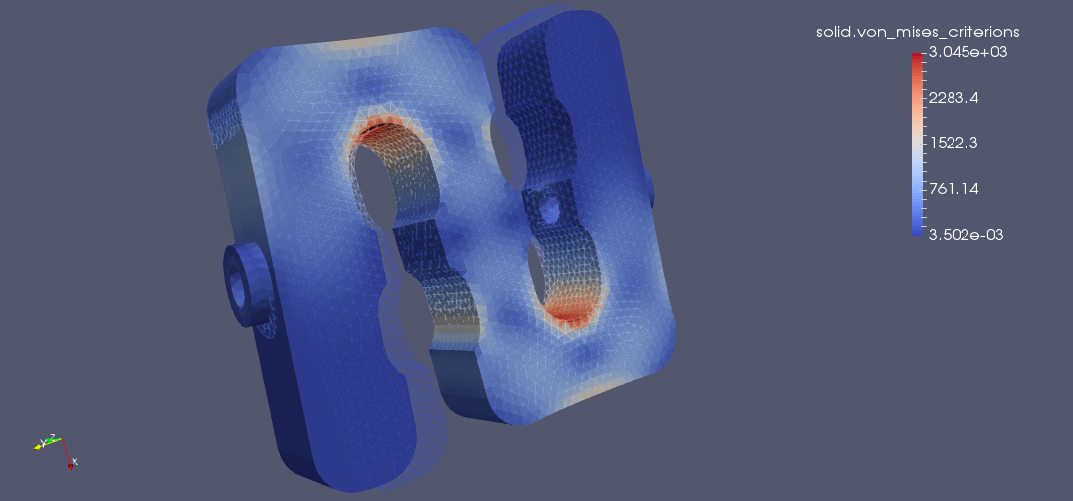
On the displacement and stress diagrams, it can be clearly seen that this object is perfectly suited as a sensor.

Plot the max of the von-mises criterion over time

fig = go.Figure()
fig.add_trace(go.Scatter(x=df["time"], y=df["Statistics_von-mises_max"],name="max"))
fig.add_trace(go.Scatter(x=df["time"], y=df["Statistics_von-mises_min"],name="min"))
fig.add_trace(go.Scatter(x=df["time"], y=df["Statistics_von-mises_mean"],name="mean"))
fig.update_layout(legend_title_text='Von-Mises min,mean and max over time')
fig.show()

Results

minmaxvonmises

6.3. 3D Model

this section is available only in html, it is not supported in jupyter notebooks. It displays the 3D model of the object.