 .pdf
.pdf
Example : Electronic component cooling
This test case has been proposed by Annabelle Le-Hyaric and Michel Fouquembergh formerly at AIRBUS.
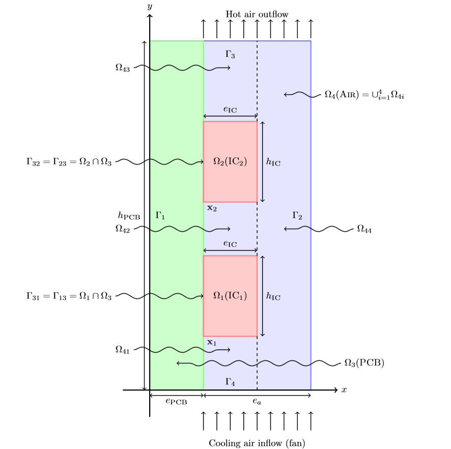
We consider a 2D model representative of the neighboring of an electronic component submitted to a cooling air flow. It is described by four geometrical domains in \(\mathbb{R}^2\) named \(\Omega_i,i=1,2,3,4\), see figure. We suppose the velocity \(\vec{v}\) is known in each domain --- for instance in \(\Omega_4\) it is the solution of previous Navier-Stokes computations. --- The temperature \(T\) of the domain \(\Omega = \cup_{i=1}^4 \Omega_i\) is then solution of heat transfer equation :
where \(t\) is the time and in each sub-domain \(\Omega_i\), \(\rho C_i\) is the volumic thermal capacity, \(k_i\) is thermal conductivity and \(Q_i\) is a volumic heat dissipated.
One should notice that the convection term in heat transfer equation may lead to spatial oscillations which can be overcome by Petrov-Galerkin type or continuous interior penalty stabilization techniques.
Integrated circuits (ICs) (domains \(\Omega_1\) and \(\Omega_2\) ) are respectively soldered on PCB at \(\mathbf{x1}=(e_{Pcb}, h_1)\) and \(\mathbf{x_2}=(e_{Pcb}, h_2)\). They are considered as rectangles with width \(e_{IC}\) and height \(h_{IC}\). The printed circuit board (PCB) is a rectangle \(\Omega_3\) of width \(e_{PCB}\) and height \(h_{PCB}\). The air(Air) is flowing along the PCB in domain \(\Omega_4\). Speed in the air channel \(\Omega_4\) is supposed to have a parabolic profile function of \(x\) coordinate. Its expression is simplified as follows (notice that \(\vec{v}\) is normally solution of Navier-Stokes equations; the resulting temperature and velocity fields should be quite different from that simplified model), we have for all \(0 \leq y \leq h_{PCB}\)
where \(f\) is a function of time modelling the starting of the PCB ventilation, i. e.
\(D\) is the air flow rate, see table~\vref{tab:1} and \(\vec{y}=(0, 1)^T\) is the unit vector along the \(y\) axis. A quick verification shows that
The medium velocity \(\vec{v}_i = \vec{0}, i=1,2,3\) in the solid domains \(\Omega_i, i=1,2,3\).
ICs dissipate heat, we have respectively
where \(Q\) is defined in table~\vref{tab:1}.
We shall denote \(\vec{n}_{|{\Omega_i}} = \vec{n}_i\) denotes the unit outward normal to \(\Omega_i\) and \(\vec{n}_{|{\Omega_j}} = \vec{n}_j\) denotes the unit outward normal to \(\Omega_j\).
1. Boundary conditions
We set
-
on \(\Gamma_3 \cap \Omega_3\), a zero flux (Neumann-like) condition
-
on \(\Gamma_3 \cap \Omega_4\), a zero flux (Robin-like) condition
-
on \(\Gamma_4, (0 \leq x \leq e_{Pcb}+e_a, y=0)\) the temperature is set (Dirichlet condition)
-
between \(\Gamma_1\) and \(\Gamma_2\), periodic conditions
-
at interfaces between the ICs and PCB, there is a thermal contact conductance:
-
on other internal boundaries, the coontinuity of the heat flux and temperature, on \(\Gamma_{ij} = \Omega_i \cap \Omega_j \neq \emptyset\)
2. Initial condition
At \(t=0s\), we set \(T = T_0\).
2.1. Inputs
The table displays the various fixed and variables parameters of this test-case.
Name |
Description |
Nominal Value |
Range |
Units |
Parameters |
||||
\(t\) |
time |
\([0, 1500\)] |
\(s\) |
|
\(Q\) |
heat source |
\(10^{6}\) |
\([0, 10^{6}\)] |
\(W \cdot m^{-3}\) |
IC Parameters |
||||
\(k_1 = k_2 = k_{IC}\) |
thermal conductivity |
\(2\) |
\([0. 2,150 \)] |
\(W \cdot m^{-1} \cdot K^{-1}\) |
\(r_{13} = r_{23} = r\) |
thermal conductance |
\(100\) |
\([10^{-1},10^{2} \)] |
\(W \cdot m^{-2} \cdot K^{-1}\) |
\(\rho C_{IC}\) |
heat capacity |
\(1. 4 \cdot 10^{6}\) |
\(J \cdot m^{-3} \cdot K^{-1}\) |
|
\(e_{IC}\) |
thickness |
\(2\cdot 10^{-3}\) |
\(m\) |
|
\(h_{IC} = L_{IC}\) |
height |
\(2\cdot 10^{-2}\) |
\(m\) |
|
\(h_{1}\) |
height |
\(2\cdot 10^{-2}\) |
\(m\) |
|
\(h_{2}\) |
height |
\(7\cdot 10^{-2}\) |
\(m\) |
|
PCB Parameters |
||||
\(k_3 = k_{Pcb}\) |
thermal conductivity |
\(0. 2\) |
\(W \cdot m^{-1} \cdot K^{-1}\) |
|
\(\rho C_{3}\) |
heat capacity |
\(2 \cdot 10^{6}\) |
\(J \cdot m^{-3} \cdot K^{-1}\) |
|
\(e_{Pcb}\) |
thickness |
\(2\cdot 10^{-3}\) |
\(m\) |
|
\(h_{Pcb}\) |
height |
\(13\cdot 10^{-2}\) |
\(m\) |
|
Air Parameters |
||||
\(T_0\) |
Inflow temperature |
\(300\) |
\(K\) |
|
\(D\) |
Inflow rate |
\(7\cdot 10^{-3}\) |
\([5 \cdot 10^{-4} ,10^{-2}\)] |
\(m^2 \cdot s^{-1}\) |
\(k_4 \) |
thermal conductivity |
\(3 \cdot 10^{-2}\) |
\(W \cdot m^{-1} \cdot K^{-1}\) |
|
\(\rho C_{4}\) |
heat capacity |
\(1100\) |
\(J \cdot m^{-3} \cdot K^{-1}\) |
|
\(e_{a}\) |
thickness |
\(4\cdot 10^{-3}\) |
\([2. 5 \cdot 10^{-3} , 5 \cdot 10^{-2}\)] |
\(m\) |
2.2. Outputs
The outputs are (i) the mean temperature \(s_1(\mu)\) of the hottest IC
and (ii) mean temperature \(s_2(\mu)\) of the air at the outlet
both depends on the solution of \eqref{eq:1} and are dependent on the parameter set \(\mu\).
We need to monitor \(s_1(\mu)\) and \(s_2(\mu)\) because \(s_1(\mu)\) is the hottest part of the model and the IC can’t have a temperature above \(340K\). \(s_2(\mu)\) is the outlet of the air and in an industrial system we can have others components behind this outlet. So the temperature of the air doesn’t have to be high to not interfere the proper functioning of these.
Testcases
We have some results from an other simulation software for this problem with methods, but we use them for an exemple purpose because Feel++ toolboxes do not handle yet the periodic conditions and the discontinuities in the toolboxes.
1. Test 1-a
This test is the base of all of the other tests, we bold the changes in the next tests. Only these parameters varies in these tests :
-
The flow rate of the system.
-
The characteristic length of the mesh.
-
The triangle family used.
-
The temporal scheme (Backward Differentiation Formula or none).
-
The stabilisation method (Galerkine Least Square or none).
The test 2 is not implemented because it is the only one that require the discontinuities on the ICs.
Flow rate |
\(7 \cdot 10^{-3}\) |
Characteristic length |
\(5 \cdot 10^{-4}\) |
Triangle family |
P1 |
Temporal scheme |
BDF 1, \(\Delta t = 1s\) |
Stabilisation |
GLS |
As the periodicity helps to dissipate the heat in both directions of the PCB, the reference results are attended to be lower than the results obtained with Feel++ on these testcases.
The Feel++ toolboxes are configured with two complementary files, the .json file configure the specific materials related to the toolbox for the geometry. The .cfg file configure the generic options, for instance the mesh file, the output directory or the solver. The .json file is common to all examples, except the stationary problem.
// -*- mode: javascript -*-
{
    "Name"      : "Eads",
    "ShortName" : "Eads",

    "Materials" : {
        "Pcb" : {
            "markers" : "Pcb",
            "name"    : "Pcb",
            "rho"     : "1.",
            "k"       : "0.2",
            "Cp"      : "2e6"
        },
        "IC1" : {
            "markers" : "IC1",
            "name"    : "IC1",
            "rho"     : "1.",
            "k"       : "2",
            "Cp"      : "1.4e6"
        },
        "IC2" : {
            "markers" : "IC2",
            "name"    : "IC2",
            "rho"     : "1.",
            "k"       : "2",
            "Cp"      : "1.4e6"
        },
        "Air" : {
            "markers" : "Air",
            "name"    : "Air",
            "rho"     : "1.",
            "k"       : "3e-2",
            "Cp"      : "1100"
        }
    },

    "BoundaryConditions" : {
        "temperature" : {
            "Dirichlet" : {
                "Air/Input"           : { "expr" : "300" },
                "Pcb/Input"           : { "expr" : "300" }
            },
            "Neumann" : {
                "Air/Output"          : { "expr" : "0" },
                "Pcb/Output"          : { "expr" : "0" },
                "Air/Right"           : { "expr" : "0" },
                "Pcb/Left"            : { "expr" : "0" }
            },
            "VolumicForces" : {
                "IC1"                 : { "expr" : "1e6*(1-exp(-t)):t" },
                "IC2"                 : { "expr" : "1e6*(1-exp(-t)):t" }
            }
        }
    },

    "InitialConditions" : {
        "temperature" : {
            "" : {
                "" : { "expr" : "300" }
            }
        }
    },

    "PostProcess" : {
        "Exports" : {
            "fields" : [
                "temperature",
                "pid"
            ]
        }
    }
}directory=toolboxes/heat/opus/test1a
case.dimension=2
[heat]
filename=$cfgdir/eads_normal.json
mesh.filename=$cfgdir/eads.geo
gmsh.hsize=5e-4
# /!\ Geometric dependant
# velocity-convection={0,(2e-3+2e-3<x)*(x<2e-3+4e-3)*7e-3*(3/2/(4e-3-2e-3))*(1-((x-(4e-3+2e-3)/2-2e-3)/((4e-3-2e-3)/2))^2)}:x
velocity-convection={0,(2e-3+2e-3<x)*(x<2e-3+4e-3)*7e-3*(3/2/(4e-3-2e-3))*(1-((x-(4e-3+2e-3)/2-2e-3)/((4e-3-2e-3)/2))^2)*(1-exp(-t/3))}:x:t
# verbose=1
# verbose_solvertimer=1
# reuse-prec=1
pc-type=lu
do_export_all=1
stabilization-gls=1
[heat.bdf]
order=1
[ts]
time-step=1
time-final=1500
# restart.at-last-save=trueThis is the basis of the other configurations files. You can download files from Github here : test1a.cfg and eads_normal.cfg, from Github . Moreover, as the toolboxes can use testcases directly from Github, you can execute this test by typing the following command :
feelpp_toolbox_heat --case "github:{repo:toolbox,path:examples/modules/heat/examples/opus}" --case.config-file test1a.cfgAll the tests follow the same command, and don’t forget to define the FEELPP_GITHUB_TOKEN, else Github can refuse the access.
2. Test 1-b
Flow rate |
\(7 \cdot 10^{-3}\) |
Characteristic length |
\(1 \cdot 10^{-3}\) |
Triangle family |
P1 |
Temporal scheme |
BDF 1, \(\Delta t = 1s\) |
Stabilisation |
GLS |
Changes :
[heat]
gmsh.hsize=1e-3
You can download files from here : test1b.cfg and eads_normal.cfg.
feelpp_toolbox_heat --case "github:{repo:toolbox,path:examples/modules/heat/examples/opus}" --case.config-file test1b.cfg3. Test 1-c
Flow rate |
\(7 \cdot 10^{-3}\) |
Characteristic length |
\(2 \cdot 10^{-4}\) |
Triangle family |
P1 |
Temporal scheme |
BDF 1, \(\Delta t = 1s\) |
Stabilisation |
GLS |
Changes :
[heat]
gmsh.hsize=2e-4
You can download files from here : test1c.cfg and eads_normal.cfg.
feelpp_toolbox_heat --case "github:{repo:toolbox,path:examples/modules/heat/examples/opus}" --case.config-file test1c.cfg4. Test 1-d
Flow rate |
\(7 \cdot 10^{-3}\) |
Characteristic length |
\(1 \cdot 10^{-4}\) |
Triangle family |
P1 |
Temporal scheme |
BDF 1, \(\Delta t = 1s\) |
Stabilisation |
GLS |
Changes :
[heat]
gmsh.hsize=1e-4
You can download files from here : test1d.cfg and eads_normal.cfg.
feelpp_toolbox_heat --case "github:{repo:toolbox,path:examples/modules/heat/examples/opus}" --case.config-file test1d.cfg5. Test 1-e
Flow rate |
\(7 \cdot 10^{-3}\) |
Characteristic length |
\(5 \cdot 10^{-4}\) |
Triangle family |
P2 |
Temporal scheme |
BDF 1, \(\Delta t = 1s\) |
Stabilisation |
GLS |
Changes :
case.discretization=P2You can download files from here : test1e.cfg and eads_normal.cfg.
feelpp_toolbox_heat --case "github:{repo:toolbox,path:examples/modules/heat/examples/opus}" --case.config-file test1e.cfg6. Test 1-f
Flow rate |
\(7 \cdot 10^{-3}\) |
Characteristic length |
\(5 \cdot 10^{-4}\) |
Triangle family |
P1 |
Temporal scheme |
BDF 2, \(\Delta t = 1s\) |
Stabilisation |
GLS |
Changes :
[heat.bdf]
order=2
feelpp_toolbox_heat --case "github:{repo:toolbox,path:examples/modules/heat/examples/opus}" --case.config-file test1f.cfgYou can download files from here : test1f.cfg and eads_normal.cfg.
7. Test 1-g
Flow rate |
\(7 \cdot 10^{-3}\) |
Characteristic length |
\(5 \cdot 10^{-4}\) |
Triangle family |
P1 |
Temporal scheme |
Stationary problem |
Stabilisation |
GLS |
IC2 reference results of test 1g |
322.483 °K |
Output reference results of test 1g |
310.436 °K |
IC2 example results of test 1g |
338.382 °K |
Output example results of test 1g |
312.522 °K |
The .json file also differs in this case :
{
    "BoundaryConditions" : {
        "temperature" : {
            "VolumicForces" : {
                "IC1"                 : { "expr" : "1e6" },
                "IC2"                 : { "expr" : "1e6" } // "1e6*(1-exp(-t)):t"
            }
        }
    }
}# [ts]
# time-step=1
# time-final=1500You can download files from here : test1g.cfg and eads_stationary.cfg.
feelpp_toolbox_heat --case "github:{repo:toolbox,path:examples/modules/heat/examples/opus}" --case.config-file test1g.cfg8. Test 3
Flow rate |
\(1 \cdot 10^{-3}\) |
Characteristic length |
\(5 \cdot 10^{-4}\) |
Triangle family |
P1 |
Temporal scheme |
BDF 1, \(\Delta t = 1s\) |
Stabilisation |
GLS |
Changes :
[heat]
velocity-convection={0,(2e-3+2e-3<x)*(x<2e-3+4e-3)*1e-3*(3/2/(4e-3-2e-3))*(1-((x-(4e-3+2e-3)/2-2e-3)/((4e-3-2e-3)/2))^2)*(1-exp(-t/3))}:x:t
You can download files from here : test3.cfg and eads_normal.cfg.
feelpp_toolbox_heat --case "github:{repo:toolbox,path:examples/modules/heat/examples/opus}" --case.config-file test3.cfg9. Test 4
Flow rate |
\(1 \cdot 10^{-3}\) |
Characteristic length |
\(5 \cdot 10^{-4}\) |
Triangle family |
P1 |
Temporal scheme |
BDF 1, \(\Delta t = 1s\) |
Stabilisation |
None |
Changes :
[heat]
velocity-convection={0,(2e-3+2e-3<x)*(x<2e-3+4e-3)*1e-3*(3/2/(4e-3-2e-3))*(1-((x-(4e-3+2e-3)/2-2e-3)/((4e-3-2e-3)/2))^2)*(1-exp(-t/3))}:x:t
stabilization-gls=0
You can download files from here : test4.cfg and eads_normal.cfg.
feelpp_toolbox_heat --case "github:{repo:toolbox,path:examples/modules/heat/examples/opus}" --case.config-file test4.cfg