3D thermal simulation of a building

1. Description

Based on the solution of the stationary heat equation, we create a reduced order model for the simulation of heat exchanges in a 3D building.

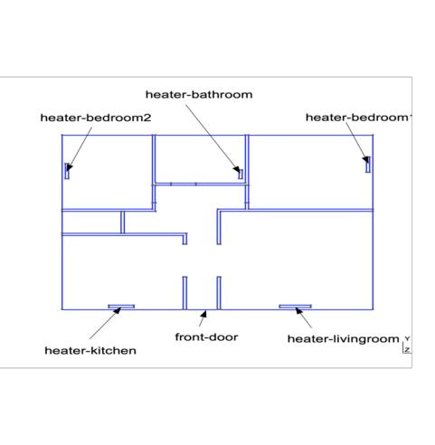
The building is composed of a corridor and 5 rooms, each of which contains a heating unit. Internal walls and doors are modelled as having finite thickness, while external walls properties (thickness and insulation) are encoded in the boundary conditions of the problem.

1.1. Mathematical model

Let \(\Omega \subset \mathbb{R}^3\) be the region occupied by the building, and denote \(\Omega_i\), \(i=0,1,2\) its subregions occupied by the air, the internal walls and the internal doors, such that \(\Omega = \cup_{i=0}^2 \Omega_i\). Let \(k_i\) be the thermal conductivities associated with the subregions.

The external boundary of the domain \(\partial \Omega\) is decomposed into two parts: \(\partial \Omega_{ext}\), which corresponds to external walls, and \(\partial \Omega_D\) which corresponds to the front door. We denote by \(\Gamma_i\) the boundary of the \(i-\)th heating unit, \(i=0,...,4\). The problem writes as

\[\begin{equation} \begin{aligned} - \nabla \cdot (k_i\nabla u) &= 0, \quad &\text{on }\Omega_i \\ u &= \mu_i \quad &\text{on }\Gamma_i, i=0,...,4, \\ - k_0 \nabla u \cdot \vec{n} &= \mu_6 (u - \mu_5), \quad &\text{on }\partial \Omega_{ext},\\ - k_0 \nabla u \cdot \vec{n} &= \sigma (u - \mu_5), \quad &\text{on }\partial \Omega_{D}. \end{aligned} \end{equation}\]

where \(\sigma\) is the convective heat exchange coefficient associated with the front door.

The parameters \(\mu_i\) correspond to

\(\mu_i \in (300,340)\), for \(i=0,...,4\), are the surface temperatures of the heating units (in Kelvin);
\(\mu_5 \in (270,290)\) is the external temperature (in Kelvin);
\(\mu_6\) is a function of the external wall thickness. The wall is composed of two layers: a cinder layer of thickness \(l_{cinder} \in (0.1,0.3) m\) and an insulation layer of thickness \(l_{insulation} \in (0.1,0.2) m\), and

\[\mu_6 = \frac{1}{0.06 + \frac{0.01}{0.5} + \frac{l_{cinder}}{0.8} + \frac{l_{insulation}}{0.032} + \frac{0.016}{0.313} + 0.14}.\]

1.2. Construction of the affine decomposition

The problem presents an affine dependence on the parameters, hence we can explicity compute the terms of the correspondent affine decomposition

\[\sum_{i = 0}^{N_A} \theta^A_i(\mu) A_i(u,v) = \sum_{j = 0}^{N_F} \theta^F_j(\mu) F_j(v),\]

where \(N_A = 1\) and \(N_F = 6\).

The first product on the left-hand side is given by \(\theta^A_0(\mu) = 1\) and

\[\begin{equation} \begin{aligned} A_0(u,v) &= \sum_{i=0}^{N_m} \int_{\Omega_i} k_i \nabla u \cdot \nabla v + \\ & - \int_{\partial \Omega_{ext}} k_0 (\nabla u v + \nabla v u )\cdot \vec{n} + \\ & + \int_{\partial \Omega_{ext}} k_0 \frac{\gamma}{h} u v +\\ & + \int_{\partial \Omega_D} uv, \end{aligned} \end{equation}\]

where \(\gamma\) is the Nitsche penalty parameter and \(h\) is the local mesh size.

The second product is given by \(\theta^A_1(\mu) = \mu_6\) and

\[A_1(u,v) = \int_{\partial \Omega_{ext}} u v.\]

The terms on the right-hand side are \(\theta^F_i(\mu) = \mu_i\) for \(i=0,...,4\), corresponding to the temperatures of the heating units, \(\theta^F_5(\mu) = \mu_5\mu_6\), corresponding to the temperature on the internal surface of the external walls, and \(\theta^F_6(\mu) = \mu_5\), corresponding to the external temperature. The corresponding linear forms are

\[\begin{equation} \begin{aligned} F_i (v) &= k_0 \int_{\Gamma_i} -\nabla v \cdot \vec{n} + \frac{\gamma}{h} v, \quad i = 0,...,4\\ F_5 (v) &= \int_{\partial \Omega_{ext}} v,\\ F_6 (v) &= \int_{\partial \Omega_D} \sigma v. \end{aligned} \end{equation}\]

1.3. Geometry

The geometry file can be found in Github here.

2. Output

The output corresponds to the air mean temperature, and it is computed as

\[\begin{equation} s(\mu) = \frac{1}{|\Omega_0|} \int_{\Omega_0} u. \end{equation}\]

3. Parameters

The table displays the various fixed and variables parameters of this test-case.

Table 1. Table of model order reduction parameters
Name	Description	Range	Units
\(\mu_0\)	Heater temperature living room	\([300,340\)]	\(K\)
\(\mu_1\)	Heater temperature kitchen	\([300,340\)]	\(K\)
\(\mu_2\)	Heater temperature bedroom 1	\([300,340\)]	\(K\)
\(\mu_3\)	Heater temperature bedroom 2	\([300,340\)]	\(K\)
\(\mu_4\)	Heater temperature bathroom	\([300,340\)]	\(K\)
\(\mu_5\)	External temperature	\([270,290\)]	\(K\)
\(\mu_6\)	Exchange coefficient external walls

Table 2. Table of constant parameters
Name	Description	Value
\(\gamma\)	Boundary conditions using Nitsche method	\(10\)
\(k_0\)	Air conductivity	\(1\)
\(k_1\)	Conductivity - internal walls	\(0.25\)
\(k_2\)	Conductivity - internal doors	\(0.13\)
\(\sigma\)	Heat transfer coefficient - front door	\(\frac{1.0}{0.06+\frac{0.06}{0.150}+\frac{0.1}{0.029}+0.14}\)

4. Setup for the notebook simulation

Setup the variables for the notebook simulation

girder_path = "https://girder.math.unistra.fr/api/v1/item/64d60522b0e9570499e1eaa1/download"
fpp_name = 'thermalbuilding.fpp'
time = 0

Results