 .pdf
.pdf
Opus Heat
This test case has been proposed by Annabelle Le-Hyaric and Michel Fouquembergh formerly at AIRBUS.
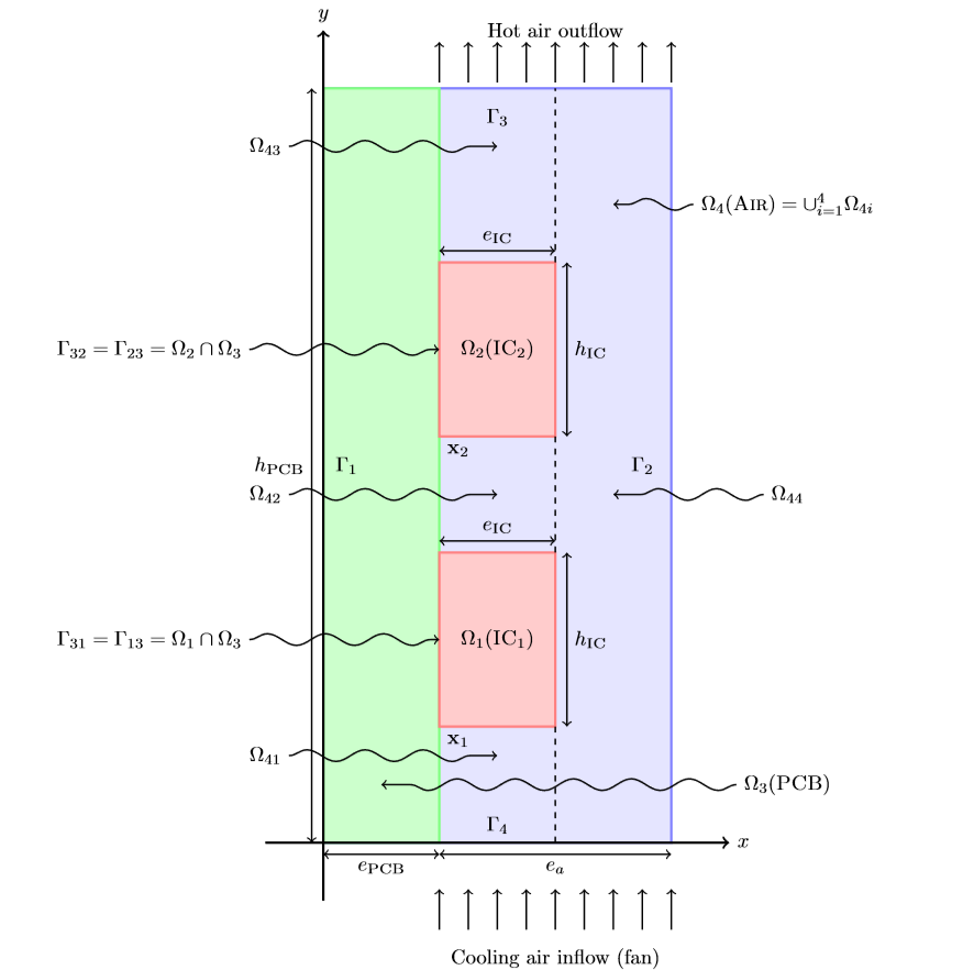
We consider a 2D model representative of the neighboring of an electronic component submitted to a cooling air flow. It is described by four geometrical domains in \(\mathbb{R}^2\) named \(\Omega_i,i=1,2,3,4\), see figure. We suppose the velocity \(\vec{v}\) is known in each domain --- for instance in \(\Omega_4\) it is the solution of previous Navier-Stokes computations. --- The temperature \(T\) of the domain \(\Omega = \cup_{i=1}^4 \Omega_i\) is then solution of heat transfer equation :
where \(t\) is the time and in each sub-domain \(\Omega_i\), \(\rho C_i\) is the volumic thermal capacity, \(k_i\) is the thermal conductivity. \(k_1\) and \(k_2\) are parameters of the model.
ICs dissipate heat, so the volumic heat dissipated \(Q_1\) and \(Q_2\) are also parameters of the model, while \(Q_3=Q_4=0\).
One should notice that the convection term in heat transfer equation may lead to spatial oscillations which can be overcome by Petrov-Galerkin type or continuous interior penalty stabilization techniques.
Integrated circuits (ICs) (domains \(\Omega_1\) and \(\Omega_2\) ) are respectively soldered on PCB at \(\mathbf{x1}=(e_{Pcb}, h_1)\) and \(\mathbf{x_2}=(e_{Pcb}, h_2)\). They are considered as rectangles with width \(e_{IC}\) and height \(h_{IC}\). The printed circuit board (PCB) is a rectangle \(\Omega_3\) of width \(e_{PCB}\) and height \(h_{PCB}\). The air(Air) is flowing along the PCB in domain \(\Omega_4\). Speed in the air channel \(\Omega_4\) is supposed to have a parabolic profile function of \(x\) coordinate. Its expression is simplified as follows (notice that \(\vec{v}\) is normally solution of Navier-Stokes equations; the resulting temperature and velocity fields should be quite different from that simplified model), we have for all \(0 \leq y \leq h_{PCB}\)
where V is a parameter of the model.
The medium velocity \(\vec{v}_i = \vec{0}, i=1,2,3\) in the solid domains \(\Omega_i, i=1,2,3\).
1. Boundary conditions
We set
-
on \(\Gamma_1\cup\Gamma_3\), a zero flux (Neumann-like) condition
-
on \(\Gamma_2\), a heat transfer (Robin-like) condition
where \(h\) is a parameter of the model
-
on \(\Gamma_4\) the temperature is set (Dirichlet condition)
-
on other internal boundaries, the coontinuity of the heat flux and temperature, on \(\Gamma_{ij} = \Omega_i \cap \Omega_j \neq \emptyset\)
3. Outputs
The output is the mean temperature \(s_1(\mu)\) of the hottest IC
4. Parameters
The table displays the various fixed and variables parameters of this test-case.
Name |
Description |
Range |
Units |
\(k_1\) |
thermal conductivity |
\([1,3\)] |
\(W \cdot m^{-1} \cdot K^{-1}\) |
\(k_2\) |
thermal conductivity |
\([1,3\)] |
\(W \cdot m^{-1} \cdot K^{-1}\) |
\(h\) |
transfer coefficient |
\([0.1,5\)] |
\(W \cdot m^{-2} \cdot K^{-1}\) |
\(Q_1\) |
heat source |
\([10^4, 10^{6}\)] |
\(W \cdot m^{-3}\) |
\(Q_1\) |
heat source |
\([10^4, 10^{6}\)] |
\(W \cdot m^{-3}\) |
\(V\) |
Inflow rate |
\([1,30\)] |
\(m^2 \cdot s^{-1}\) |
Name |
Description |
Nominal Value |
Units |
\(t\) |
time |
\([0, 500\)] |
\(s\) |
\(T_0\) |
initial temperature |
\(300\) |
\(K\) |
IC Parameters |
|||
\(\rho C_{IC}\) |
heat capacity |
\(1.4 \cdot 10^{6}\) |
\(J \cdot m^{-3} \cdot K^{-1}\) |
\(e_{IC}\) |
thickness |
\(2\cdot 10^{-3}\) |
\(m\) |
\(h_{IC} = L_{IC}\) |
height |
\(2\cdot 10^{-2}\) |
\(m\) |
\(h_{1}\) |
height |
\(2\cdot 10^{-2}\) |
\(m\) |
\(h_{2}\) |
height |
\(7\cdot 10^{-2}\) |
\(m\) |
PCB Parameters |
|||
\(k_3 = k_{Pcb}\) |
thermal conductivity |
\(0. 2\) |
\(W \cdot m^{-1} \cdot K^{-1}\) |
\(\rho C_{3}\) |
heat capacity |
\(2 \cdot 10^{6}\) |
\(J \cdot m^{-3} \cdot K^{-1}\) |
\(e_{Pcb}\) |
thickness |
\(2\cdot 10^{-3}\) |
\(m\) |
\(h_{Pcb}\) |
height |
\(13\cdot 10^{-2}\) |
\(m\) |
Air Parameters |
|||
\(T_0\) |
Inflow temperature |
\(300\) |
\(K\) |
\(k_4 \) |
thermal conductivity |
\(3 \cdot 10^{-2}\) |
\(W \cdot m^{-1} \cdot K^{-1}\) |
\(\rho C_{4}\) |
heat capacity |
\(1100\) |
\(J \cdot m^{-3} \cdot K^{-1}\) |
\(e_{a}\) |
thickness |
\(4\cdot 10^{-3}\) |
\(m\) |