 .pdf
.pdf
Quick Start with Docker
1. Installation Quick Start
Using Feel++ inside Docker is the recommended and fastest way to use Feel++.
We strongly encourage you to follow the Docker installation steps if you begin with Feel++ in particular as an end-user.
2. Usage Quick Start
Start the main Feel++ Docker container feelpp/feelpp-toolboxes` as follows
$ docker run -it --rm -e LOCAL_USER_ID=`id -u $USER` -v $HOME/feel:/feel feelpp/feelpp-toolboxes
simply copy-paste the command line in your terminal to start the feelpp/feelpp-toolboxes container.
|
Here are some explanations about the different parts in the command line
$ docker (1)
  run (2)
  -it (3)
  --rm (4)
  -e LOCAL_USER_ID=`id -u`(5)
  -v $HOME/feel:/feel (6)
feelpp/feelpp-toolboxes (7)| 1 | docker is the application that allows to create and execute Containers |
| 2 | run allows to execute the image feelpp/feelpp-toolboxes |
| 3 | the option -it runs Docker in interactive mode; |
| 4 | the option --rm makes sure that the container is deleted after the user exits Docker |
| 5 | we need to pass your user id to Docker so that the data you generate from Docker belongs to you; |
| 6 | maps the directory $HOME/feel on your host to /feel in Docker, Feel++ write in /feel the results of the simulations. Passing your id, i.e LOCAL_USER_ID, allows to ensure that the generated data on Feel++ belongs to you on your host system; |
| 7 | execute the image feelpp/feelpp-toolboxes and create the associated container . |
Then run e.g. the Quickstart Laplacian that solves the Laplacian problem in Running the quickstart Laplacian in sequential or in Quickstart Laplacian on 4 cores in parallel.
Several testcases (configuration files) have been installed in /feel/testcases (in Docker container) or $HOME/feel/testcases once you have executed the command line above.
|
$ feelpp_qs_laplacian_2d --config-file /feel/testcases/quickstart/laplacian/feelpp2d/feelpp2d.cfg> feelpp_qs_laplacian_2d (1)
--config-file /feel/testcases/quickstart/laplacian/feelpp2d/feelpp2d.cfg(2)| 1 | executable to run |
| 2 | configuration file (text) to setup the problem : mesh, material properties and boundary conditions |
The results are stored in Docker in
/feel/qs_laplacian/feelpp2d/np_1/exports/ensightgold/qs_laplacian/
and on your computer
$HOME/feel/qs_laplacian/feelpp2d/np_1/exports/ensightgold/qs_laplacian/
The mesh and solutions can be visualized using e.g. Paraview or Visit.
|
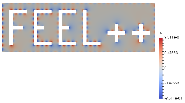
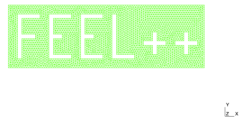
> mpirun -np 4 feelpp_qs_laplacian_2d --config-file /feel/testcases/quickstart/laplacian/feelpp2d/feelpp2d.cfgThe results are stored in a simular place as above: just replace np_1 by np_4 in the paths above. The results should look like
|
|
Solution |
Mesh |
3. Syntax Start
Here are some excerpts from Quickstart Laplacian that solves the Laplacian problem. It shows some of the features of Feel++ and in particular the domain specific language for Galerkin methods.
First we load the mesh, define the function space define some expressions
    tic();
    auto mesh = loadMesh(_mesh=new Mesh<Simplex<FEELPP_DIM,1>>);
    toc("loadMesh");

    tic();
    auto Vh = Pch<2>( mesh ); (1)
    auto u = Vh->element("u"); (2)
    auto mu = expr(soption(_name="functions.mu")); // diffusion term (3)
    auto f = expr( soption(_name="functions.f"), "f" ); (4)
    auto r_1 = expr( soption(_name="functions.a"), "a" ); // Robin left hand side expression (5)
    auto r_2 = expr( soption(_name="functions.b"), "b" ); // Robin right hand side expression (6)
    auto n = expr( soption(_name="functions.c"), "c" ); // Neumann expression (7)
    auto solution = expr( checker().solution(), "solution" ); (8)
    auto g = checker().check()?solution:expr( soption(_name="functions.g"), "g" ); (9)
    auto v = Vh->element( g, "g" ); (3)
    toc("Vh");
Second we define the linear and bilinear forms to solve the problem
    tic();
    auto l = form1( _test=Vh );
    l = integrate(_range=elements(mesh),
                  _expr=f*id(v));
    l+=integrate(_range=markedfaces(mesh,"Robin"), _expr=r_2*id(v));
    l+=integrate(_range=markedfaces(mesh,"Neumann"), _expr=n*id(v));
    toc("l");

    tic();
    auto a = form2( _trial=Vh, _test=Vh);
    tic();
    a = integrate(_range=elements(mesh),
                  _expr=mu*inner(gradt(u),grad(v)) );
    toc("a");
    a+=integrate(_range=markedfaces(mesh,"Robin"), _expr=r_1*idt(u)*id(v));
    a+=on(_range=markedfaces(mesh,"Dirichlet"), _rhs=l, _element=u, _expr=g );
    //! if no markers Robin Neumann or Dirichlet are present in the mesh then
    //! impose Dirichlet boundary conditions over the entire boundary
    if ( !mesh->hasAnyMarker({"Robin", "Neumann","Dirichlet"}) )
        a+=on(_range=boundaryfaces(mesh), _rhs=l, _element=u, _expr=g );
    toc("a");
More explanations are available in the Laplacian example.