.pdf
.pdf
Maxwell Quasi-Static Models
1. High-Field Magnets
High Field Magnets are mainly solenoidal coils, made of copper alloys, that are powered with high current (up to 33 kA in our case). To prevent excessive temperature in the magnets, a water forced flow (with a flow rate up to 30 l/s) is used to cool them down. These magnets are submitted to large Lorentz forces (arising from the coupling of the generated magnetic field \(\mathbf{B}\) and the current density \(\mathbf{j}\)) and to thermal dilatation. Typically magnet material are operated at 90\% of their elastic limit.
High Field Magnet modeling thus relies on a multi-physic approach involving:
-
Maxwell equations using the so-called MQS (aka Maxwell Quasi-Static) approximation,
-
Heat equation,
-
Elasticity/Plasticity equation,
-
Thermo-Hydraulic equations to account for the water flow.
For sake of simplicity, the cooling of the magnets is modeled as forced flow boundary conditions on the water cooled surfaces. Next we consider only the elasticity model.
The modelling of powering High Field Magnets and power failure motivates this document and the introduction of Maxwell Quasi-STatic models in Feel++.
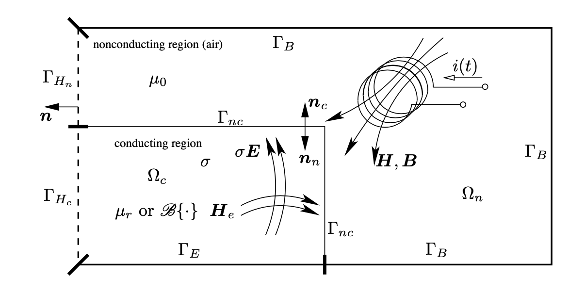
2. Eddy field current
In time varying case ( \(\partial / \partial t \neq 0\) ), the electric and the magnetic fields are coupled. Currents flowing in coils generate a magnetic field in the vicinity of the coil. The time variation of this magnetic field induces electric field that causes eddy currents flowing in conducting materials. The magnetic field generated by the eddy currents modifies the effect of sources.
A typical structure of an eddy current field problem can be seen in the Figure below. In the eddy current free region denoted by \(\Omega_{n},\) there is a magnetic field with equations
Sometimes it is filled with air \(\left(\mu=\mu_{0}, \text { or } \nu=\nu_{0}\right)\) At low frequencies and with normal conducting materials, the displacement currents are small compared with the conducting currents and they can be neglected, i.e.
Consequently, the studied electromagnetic fields can be described by the 'quasi-static' Maxwell’s equations written in differential form as