 .pdf
.pdf
2D Advection-diffusion with Taylor-Green Vortex
1. Introduction
We study the solution of a 2D advection-diffusion equation (used to model the dispersion of a contaminant) in presence of a Taylor-Green vortex \(\beta(x,t)\). The problem can be solved for different values of the diffusion coefficient \(\mu\).
2. Advection-diffusion with Taylor-Green Vortex
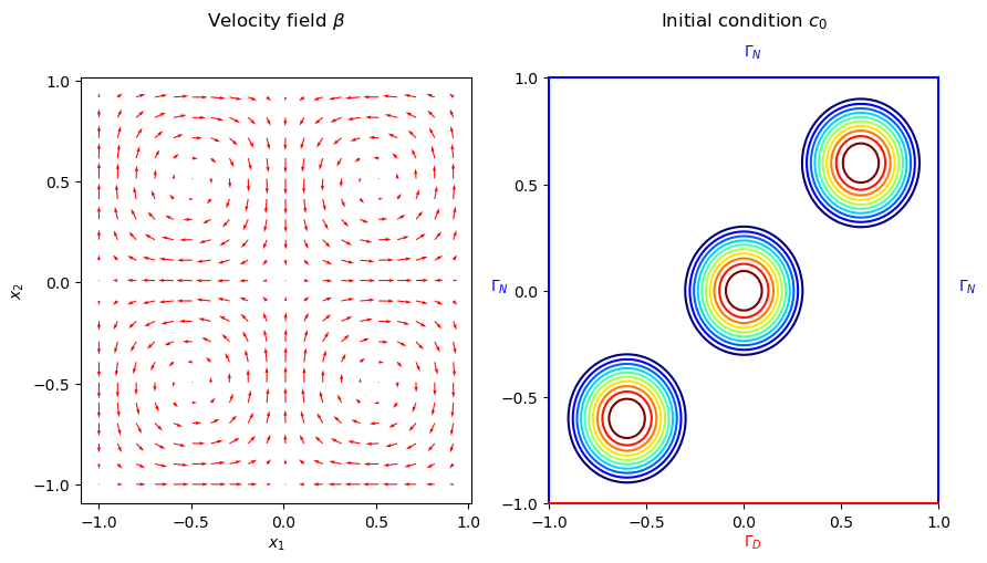
The problem is defined on the spatial domain \(\Omega = (-1, 1)^2\) with Dirichlet boundary \(\Gamma_D := (-1, 1) \times \{-1\}\) and Neumann boundary \(\Gamma_N := \partial\Omega \setminus \Gamma_D\). The governing parametric PDE (pPDE) can be described as follows:
where the velocity field \(\beta := (\sin(\pi x_1) \cos(\pi x_2), -\cos(\pi x_1) \sin(\pi x_2))^{\top}\), \(x = (x_1, x_2)\), is a solenoidal field. The initial condition, \(c_0(\cdot; \mu): \Omega \rightarrow \mathbb{R}\), is given by the sum of three Wendland functions \(\bar{\psi}_{2,1}^i\) of radius 0.4 and centers located at \((-0.6, -0.6)\), \((0, 0)\) and \((0.6, 0.6)\). The Wendland functions are radial functions with compact support on the unit ball, and \(\psi_{2,1}(r)\) has the following closed form
Appropriate transformations have been applied to \(\psi_{2,1}(r)\) in order to get the scaled and translated Wendland functions \(\bar{\psi}_{2,1}^i\).
The velocity field \(\beta\), the initial condition \(c_0(\cdot; \mu)\), and the boundaries are illustrated in the following figure.
3. Mathematical formulation for the reduced order problem
Given a value for \(\mu \in \mathcal{P} \subset \mathbb{R}^p\), we solve the weak formulation of the previous problem by finding \(c(t;\mu) \in V\) such that:
where \(V=H^1_{0, \Gamma_D}(\Omega)=\{ v \in H^1(\Omega) \mid v = 0 \text{ on } \Gamma_D \}\), and \(m(\cdot,\cdot): V \times V \rightarrow \mathbb{R}\), \(a(\cdot,\cdot;\mu): V \times V \rightarrow \mathbb{R}\) are the bilinear forms defined as:
Additionally, we are interested in a specific Output:
3.1. Affine decomposition (without boundary conditions)
The bilinear form \(a(\cdot,\cdot;\mu)\) is affine in the parameter \(\mu\), i.e.:
\(a(\cdot,\cdot;\mu) = \sum_{q=1}^{Q_a} \theta^a_q(\mu) \,a_q(\cdot,\cdot)\)
where \(a_q:V \times V \rightarrow \mathbb{R}\) are bilinear forms independent of \(\mu\) and \(\theta^a_q: \mathcal{P} \rightarrow \mathbb{R}\) are scalar quantities depending only on \(\mu\).
In particular, \(Q_a=2\) and the decomposition is given by:
where:
\(\theta^a_1(\mu) = 1 \quad \text{and} \quad \theta^a_2(\mu) = \mu\)
and:
\(a_1(u,v) = \int_{\Omega} (\beta \cdot \nabla u) \, v \, dx \quad \text{and} \quad a_2(u,v) = \int_{\Omega} \nabla u \cdot \nabla v \, dx \quad \forall u,v \in V.\)
|
In general, we seek an affine decomposition for both the bilinear form and the linear form in the variational formulation, as well as for the output functional \(\ell\). However, in our case, the right hand side linear form is equal to zero and the output functional doesn’t depend explicitly on the parameter \(\mu\). |
3.2. Affine decomposition (with boundary conditions)
A very practical approach to treat the boundary conditions (in particular Dirichlet) in the context of reduced basis method is to impose them weakly i.e. include them in the weak formulation and even in the affine decomposition of the problem as a penalisation terms. This approach is known as the Nitsche’s method. We won’t go into mathematical details that can be found in Feel++ documentation, but we will just give the final expression of the affine decomposition. First we recall that we have homogeneous Dirichlet boundary conditions on \(\Gamma_D\), and that Neumann boundary conditions are natural. Finally, we have the following affine decomposition:
where:
\(\theta^a_1(\mu) = 1 , \quad \theta^a_2(\mu) = \mu \quad \text{and} \quad h \text{ is the mesh size}\).
|
3.3. Output
We are interested in non-compliant time-dependent multiple outputs defined as follows:
\(s(t;\mu)= (s_1(t;\mu), s_2(t;\mu), s_3(t;\mu)) \quad \\ \\ \text{with} \quad s_1(t;\mu) = \int_{\Omega} c(t;\mu) \, \eta_1 dx, \quad s_2(t;\mu) = \int_{\Omega} c(t;\mu) \, \eta_2 dx \quad \text{and} \quad s_3(t;\mu) = \int_{\Omega} c(t;\mu) \, \eta_3 dx\)
where \(\eta_1, \eta_2, \eta_3\) are three Wendland functions \(\psi_{2,1}\) of radius 0.1 and centers \((0.1, 0.7), (0.1, 0.7) \text{ and } (0.5, 0.1)\) respectively.
4. Setup for the notebook simulation
import numpy as np
girder_path = "https://girder.math.unistra.fr/api/v1/item/64c165a5b0e9570499e1cc3c/download"
fpp_name = 'ad.fpp'
time = np.linspace(start=0, stop=2.5, num=251)
5. Downloading the reduced order model from Girder
The offline creation of the reduced basis has already been performed, and an archive is downloaded from Girder. It contains the basis, the model and the configuration files that are necessary for the online simulation. The following code snippet performs the download.
import requests
r=requests.get(girder_path)
with open(fpp_name,'wb') as f:
    f.write(r.content)
Results
--------------------------------------------------------------------------- NameError Traceback (most recent call last) File:2 1 import requests ----> 2 r=requests.get(girder_path) 3 with open(fpp_name,'wb') as f: 4 f.write(r.content) NameError: name 'girder_path' is not defined
6. Running the case using a Jupyter notebook
It is possible to download this page as a Jupyter notebook and run it in an environment that contains a local installation of Feel++ and its Python wrappers.
import feelpp
from feelpp.mor import *
ms=feelpp.mor.MORModels(fpp_name)
muspace = ms.parameterSpace()
sampling = muspace.sampling()
sampling.sample(4, "random")
r=ms.run(sampling,{"N":10})
Results
--------------------------------------------------------------------------- NameError Traceback (most recent call last) File:3 1 import feelpp 2 from feelpp.mor import * ----> 3 ms=feelpp.mor.MORModels(fpp_name) 4 muspace = ms.parameterSpace() 5 sampling = muspace.sampling() NameError: name 'fpp_name' is not defined
from pandas import DataFrame as df
from pandas import options as op
from pandas import set_option
outputs={}
errors={}
output_dataframes = list()
errors_dataframes = list()
for i in range(len(r)):
    outputs={}
    errors={}
    for o in range(len(r[i])):
        str_time = "Time"
        str_output = "Output "+str(o)
        str_error = "Error "+str(o)

        outputs[str_time] = time
        outputs[str_output] = np.array(r[i][o].outputs())
        outputs[str_error] = [np.array(r[i][o].errors())]


    output_frame = df(data=outputs)


    set_option('display.float_format', '{:.2E}'.format)

    output_dataframes.append(output_frame)

op.display.max_colwidth = 100

i=0
for frame in output_dataframes:
    print("Parameters :",sampling[i])
    print(frame)
    print("\n")
    i=i+1
Results
--------------------------------------------------------------------------- NameError Traceback (most recent call last) File:8 6 output_dataframes = list() 7 errors_dataframes = list() ----> 8 for i in range(len(r)): 9 outputs={} 10 errors={} NameError: name 'r' is not defined
import plotly.graph_objects as go

for i in range(len(r)):
    # Create a Plotly figure with a scatter plot
    fig = go.Figure()

    for o in range(len(r[i])):
        v=np.array(r[i][o].outputs())
        err=np.array(r[i][o].errors())

        min_values = v*(1-10/100)
        max_values = v*(1+10/100)
        # print(f"v: {v}")
        # print(f"min_values: {min_values}")
        # print(f"max_values: {max_values}")

        assert time.size == min_values.size == max_values.size == v.size

        fig.add_trace(go.Scatter(
            x=time,
            y=v,
            mode='lines+markers',
            name=f'wendland-{o}'
        ))

    # Update the layout of the figure
    fig.update_layout(
        title=f'Sensor outputs for mu={sampling[i]}',
        xaxis_title='Time',
        yaxis_title='Value',

        # Use 'category' type for the x-axis to treat it as discrete dates
        xaxis=dict(tickformat='.2f'),
    )

    # Show the plot
    fig.show()